devtools::install_github("ebenmichael/augsynth")12 - Synthetic Control (2/2)
Slides
Practical example
Augmented synthetic control
We revisit the data example from last week (slightly changed and trimmed) and apply a more advanced method for synthetic control estimation, known as the augmented synthetic control, proposed by Ben-Michael, Feller, and Rothstein, 2021. This doubly robust estimator combines elements from both the synthetic control estimator and an outcome model estimator. While it does not strictly prohibit negative weights, regularization is used to minimize their occurrence. The general idea is to assess the pre-treatment imbalance using an outcome model and then reweight the synthetic control with the new weights.
\[
\begin{align*}
\hat{Y}_{1T}^{\text{aug}}(0) &= \overbrace{\sum_{i=2}^{N+1} \hat{w}_i^{\text{sc}} Y_{iT}}^{\text{SC estimate}} + \overbrace{\left( \hat{m}_{1T} - \sum_{i=2}^{N+1} \hat{w}_i^{\text{sc}} \hat{m}_{iT} \right)}^{\text{imbalance correction}} \\
&= \underbrace{\hat{m}_{1T}}_{\text{outcome model}} + \underbrace{\sum_{i=2}^{N+1} \hat{w}_i^{\text{sc}} (Y_{iT} - \hat{m}_{iT})}_{\text{"IPW-like" re-weights to balance residuals}}
\end{align*}
\] Let’s use the augsynth() method from the augsynth package for estimation. You have to install it from GitHub, so please run the following command.
# A tibble: 6 × 11
  city    density employment   gdp population treated post  cohort revenue period     treat_post
  <chr>     <int>      <dbl> <dbl>      <dbl> <lgl>   <lgl>  <dbl>   <dbl> <date>          <int>
1 Atlanta     333      0.601  5.78       4.91 FALSE   FALSE    Inf    23.3 2009-01-01          0
2 Atlanta     333      0.601  5.78       4.91 FALSE   FALSE    Inf    24.1 2009-02-01          0
3 Atlanta     333      0.601  5.78       4.91 FALSE   FALSE    Inf    23.1 2009-03-01          0
4 Atlanta     333      0.601  5.78       4.91 FALSE   FALSE    Inf    27.6 2009-04-01          0
5 Atlanta     333      0.601  5.78       4.91 FALSE   FALSE    Inf    26.3 2009-05-01          0
6 Atlanta     333      0.601  5.78       4.91 FALSE   FALSE    Inf    28.1 2009-06-01          0
You can specify whether you want to run an outcome model and choose its form. If you opt not to use any model, the basic synthetic control method estimates will be provided. First, we will run the analysis without an outcome model, and then we will use ridge regression. However, other methods are also available. By typing ?augsynth into your console, you can see the additional options. Apart from this, the arguments are similar to those you have seen in previous weeks.
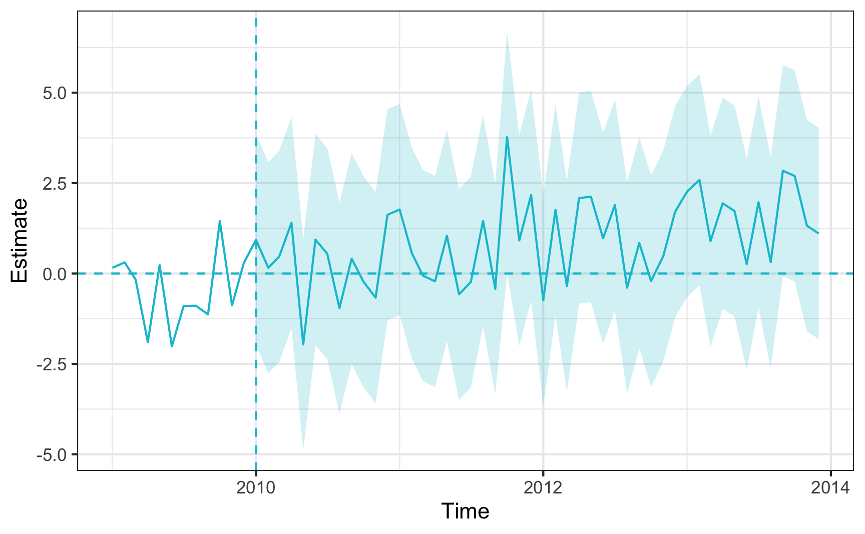
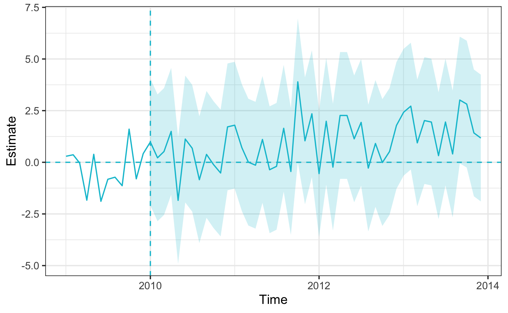
Task 1: Fill out the code below and report the results. Do it once without and once without outcome model. What is the difference? Please note, that the inference takes some time.
Code
One outcome and one treatment time found. Running single_augsynth.Code
sc_summ <- summary(att_sc)
sc_summ
Call:
single_augsynth(form = form, unit = !!enquo(unit), time = !!enquo(time),
    t_int = t_int, data = data, progfunc = "None", scm = TRUE)

Average ATT Estimate (p Value for Joint Null):  0.895   ( 0.83 )
L2 Imbalance: 3.704
Percent improvement from uniform weights: 28%

Covariate L2 Imbalance: 4.467
Percent improvement from uniform weights: 18%

Avg Estimated Bias: NA

Inference type: Conformal inference

       Time Estimate 95% CI Lower Bound 95% CI Upper Bound p Value
 2010-01-01    0.931              -1.99               3.85   0.630
 2010-02-01    0.161              -2.76               3.08   1.000
 2010-03-01    0.472              -2.45               3.39   0.638
 2010-04-01    1.403              -1.52               4.32   0.316
 2010-05-01   -1.961              -4.88               0.96   0.162
 2010-06-01    0.939              -1.98               3.86   0.630
 2010-07-01    0.546              -2.38               3.47   0.622
 2010-08-01   -0.955              -3.88               1.97   0.564
 2010-09-01    0.410              -2.51               3.33   0.618
 2010-10-01   -0.225              -3.15               2.70   0.867
 2010-11-01   -0.668              -3.59               2.25   0.631
 2010-12-01    1.625              -1.30               4.55   0.391
 2011-01-01    1.769              -1.15               4.69   0.237
 2011-02-01    0.563              -2.36               3.48   0.626
 2011-03-01   -0.058              -2.98               2.86   1.000
 2011-04-01   -0.217              -3.14               2.70   0.919
 2011-05-01    1.045              -1.88               3.97   0.629
 2011-06-01   -0.577              -3.50               2.34   0.619
 2011-07-01   -0.232              -3.15               2.69   0.856
 2011-08-01    1.456              -1.46               4.38   0.313
 2011-09-01   -0.423              -3.34               2.50   0.694
 2011-10-01    3.774               0.00               6.70   0.148
 2011-11-01    0.914              -2.01               3.83   0.607
 2011-12-01    2.169              -0.75               5.09   0.141
 2012-01-01   -0.738              -3.66               2.18   0.614
 2012-02-01    1.759              -1.16               4.68   0.227
 2012-03-01   -0.352              -3.27               2.57   0.756
 2012-04-01    2.085              -0.84               5.00   0.228
 2012-05-01    2.125              -0.80               5.05   0.216
 2012-06-01    0.973              -1.95               3.89   0.608
 2012-07-01    1.894              -1.03               4.82   0.235
 2012-08-01   -0.391              -3.31               2.53   0.586
 2012-09-01    0.846              -2.07               3.77   0.609
 2012-10-01   -0.209              -3.13               2.71   0.916
 2012-11-01    0.483              -2.44               3.40   0.621
 2012-12-01    1.707              -1.21               4.63   0.224
 2013-01-01    2.274              -0.65               5.20   0.221
 2013-02-01    2.587              -0.33               5.51   0.230
 2013-03-01    0.896              -2.02               3.82   0.623
 2013-04-01    1.943              -0.98               4.86   0.221
 2013-05-01    1.727              -1.19               4.65   0.266
 2013-06-01    0.260              -2.66               3.18   0.914
 2013-07-01    1.970              -0.95               4.89   0.224
 2013-08-01    0.312              -2.61               3.23   0.764
 2013-09-01    2.841              -0.08               5.76   0.290
 2013-10-01    2.698              -0.22               5.62   0.089
 2013-11-01    1.322              -1.60               4.24   0.618
 2013-12-01    1.105              -1.82               4.03   0.391
Code
plot(sc_summ)Code
One outcome and one treatment time found. Running single_augsynth.Code
augsc_summ <- summary(att_augsc)
augsc_summ
Call:
single_augsynth(form = form, unit = !!enquo(unit), time = !!enquo(time),
    t_int = t_int, data = data, progfunc = "Ridge", scm = TRUE)

Average ATT Estimate (p Value for Joint Null):  1   ( 0.83 )
L2 Imbalance: 3.629
Percent improvement from uniform weights: 29%

Covariate L2 Imbalance: 4.254
Percent improvement from uniform weights: 22%

Avg Estimated Bias: -0.082

Inference type: Conformal inference

       Time Estimate 95% CI Lower Bound 95% CI Upper Bound p Value
 2010-01-01    0.983             -2.086                4.1   0.596
 2010-02-01    0.217             -2.852                3.3   0.923
 2010-03-01    0.521             -2.548                3.6   0.601
 2010-04-01    1.497             -1.572                4.6   0.323
 2010-05-01   -1.844             -4.912                1.2   0.315
 2010-06-01    1.125             -1.943                4.2   0.591
 2010-07-01    0.681             -2.388                3.8   0.619
 2010-08-01   -0.843             -3.912                2.2   0.633
 2010-09-01    0.382             -2.687                3.5   0.735
 2010-10-01   -0.107             -3.176                3.0   0.938
 2010-11-01   -0.518             -3.586                2.6   0.848
 2010-12-01    1.715             -1.354                4.8   0.390
 2011-01-01    1.796             -1.273                4.9   0.245
 2011-02-01    0.706             -2.362                3.8   0.625
 2011-03-01    0.007             -3.062                3.1   1.000
 2011-04-01   -0.141             -3.210                2.9   0.920
 2011-05-01    1.105             -1.963                4.2   0.535
 2011-06-01   -0.360             -3.429                2.7   0.837
 2011-07-01   -0.196             -3.265                2.9   0.914
 2011-08-01    1.645             -1.424                4.7   0.326
 2011-09-01   -0.445             -3.514                2.6   0.849
 2011-10-01    3.894              0.000                7.0   0.151
 2011-11-01    1.040             -2.029                4.1   0.466
 2011-12-01    2.349             -0.720                5.4   0.086
 2012-01-01   -0.548             -3.617                2.5   0.678
 2012-02-01    1.986             -1.083                5.1   0.239
 2012-03-01   -0.235             -3.303                2.8   0.929
 2012-04-01    2.267             -0.801                5.3   0.245
 2012-05-01    2.266             -0.803                5.3   0.253
 2012-06-01    1.135             -1.934                4.2   0.399
 2012-07-01    1.932             -1.137                5.0   0.230
 2012-08-01   -0.281             -3.349                2.8   0.942
 2012-09-01    0.912             -2.157                4.0   0.544
 2012-10-01   -0.012             -3.081                3.1   0.907
 2012-11-01    0.521             -2.548                3.6   0.688
 2012-12-01    1.786             -1.283                4.9   0.236
 2013-01-01    2.423             -0.646                5.5   0.136
 2013-02-01    2.718             -0.351                5.8   0.238
 2013-03-01    0.941             -2.128                4.0   0.508
 2013-04-01    2.020             -1.048                5.1   0.242
 2013-05-01    1.948             -1.121                5.0   0.219
 2013-06-01    0.321             -2.748                3.4   0.848
 2013-07-01    1.950             -1.118                5.0   0.218
 2013-08-01    0.404             -2.665                3.5   0.934
 2013-09-01    3.013             -0.056                6.1   0.324
 2013-10-01    2.818             -0.251                5.9   0.083
 2013-11-01    1.422             -1.647                4.5   0.395
 2013-12-01    1.174             -1.895                4.2   0.387
Code
plot(augsc_summ)Staggered timing
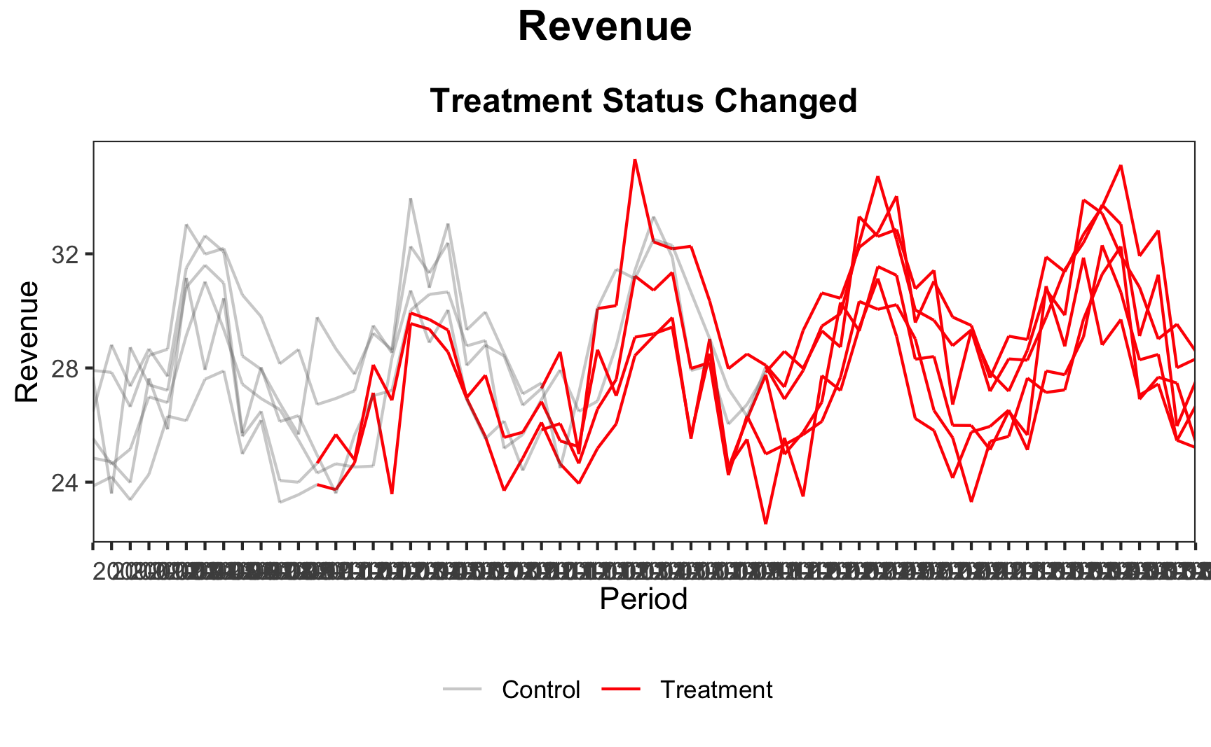
Historically, synthetic control methods have been applied to single treated units, while difference-in-differences estimators were typically used for multiple treated units and staggered treatments. However, if we are unwilling to assume parallel trends and prefer to use the synthetic control approach, we can utilize the augsynth package again.
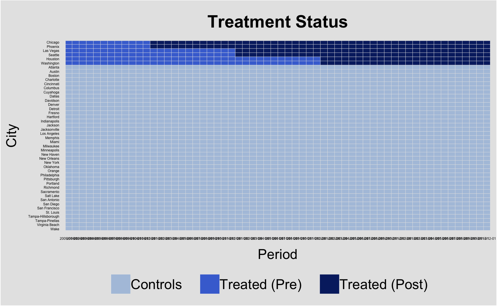
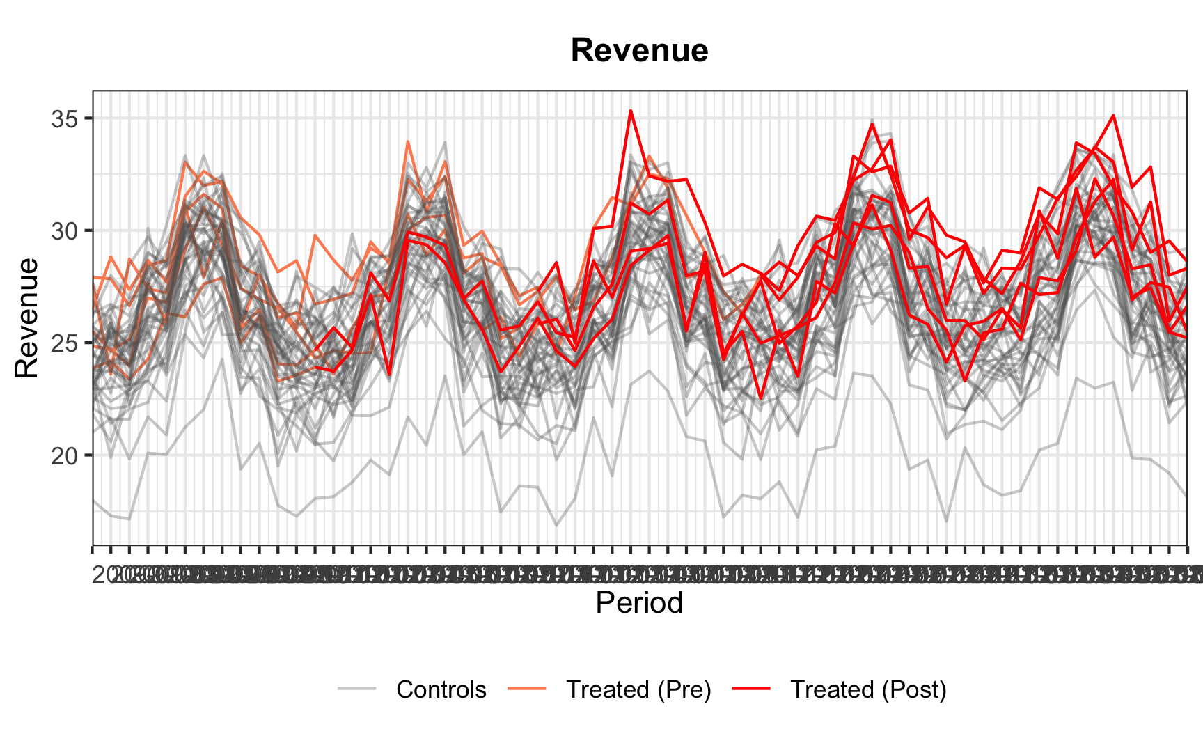
But first, let’s get the data where the new feature for the ride sharing platform were rolled out at multiple cities at different points of time and explore the data. A package that helps with visualization of staggered rollouts is panelView.
# A tibble: 6 × 15
  city     year density employment   gdp population month treated  post cohort summer pre_summer post_summer revenue period
  <chr>   <int>   <int>      <dbl> <dbl>      <dbl> <int> <lgl>   <dbl>  <dbl> <lgl>  <lgl>      <lgl>         <dbl> <date>
1 Chicago  2009     498      0.585  5.97       9.43     1 TRUE        0   2010 FALSE  FALSE      FALSE          23.9 2009-01-01
2 Chicago  2009     498      0.585  5.97       9.43     2 TRUE        0   2010 FALSE  FALSE      FALSE          24.2 2009-02-01
3 Chicago  2009     498      0.585  5.97       9.43     3 TRUE        0   2010 FALSE  FALSE      FALSE          23.4 2009-03-01
4 Chicago  2009     498      0.585  5.97       9.43     4 TRUE        0   2010 FALSE  TRUE       FALSE          24.3 2009-04-01
5 Chicago  2009     498      0.585  5.97       9.43     5 TRUE        0   2010 FALSE  TRUE       FALSE          26.3 2009-05-01
6 Chicago  2009     498      0.585  5.97       9.43     6 TRUE        0   2010 TRUE   FALSE      FALSE          26.2 2009-06-01
Task 2: Read through the tutorial and reproduce the following plots. Describe what you can see.
Code
library("panelView")

panelview(revenue ~ post,
          data = ride_multi,
          index = c("city","period"),
          xlab = "Period",
          ylab = "City",
          cex.axis = 3,
          by.timing = TRUE,
          pre.post = TRUE
          )
Code
Code
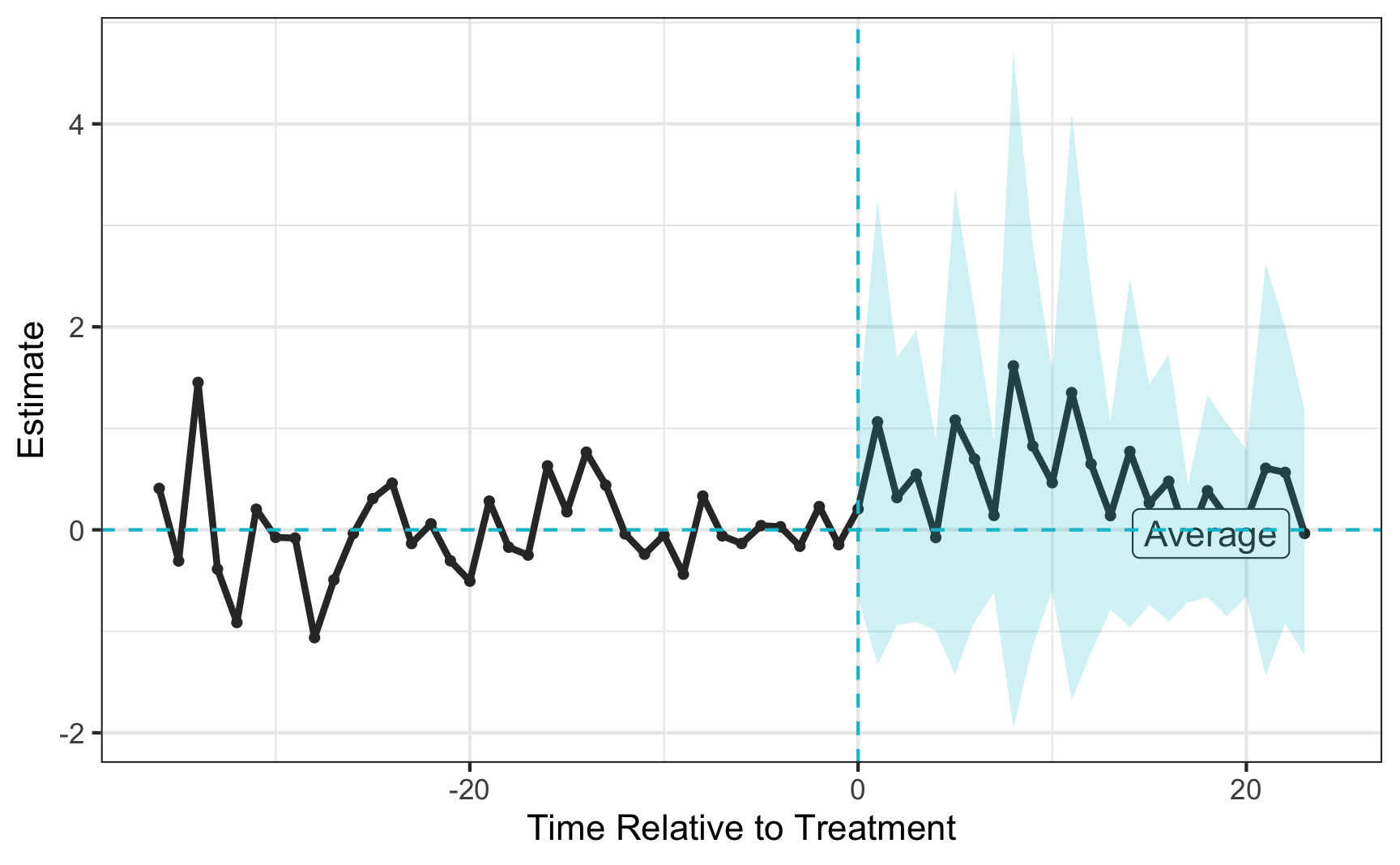
However, the problem that arises is that aggregate multiple synthetic controls into a single parameter estimate. We need to find the balance between simply estimating a synthetic control for each treated unit and pooled synthetic control for all treated units. The answer is the partially-pooled synthetic control that minimizes a weighted average of the two imbalances and includes an intercept to account for level differences.
Equation highlights two equivalent interpretations: average of unit-specific SCM estimates or SCM estimate of the average treated unit.
\[ \begin{aligned} \hat{\tau}_k = \frac{1}{J} \sum_{j=1}^J \hat{\tau}_{jk} &= \frac{1}{J} \sum_{j=1}^J \left[ Y_{jT_j + k} - \sum_{i=1}^N \hat{w}_{ij} Y_{iT_j + k} \right] \\ &= \frac{1}{J} \sum_{j=1}^J Y_{jT_j + k} - \sum_{i=1}^N \frac{1}{J} \sum_{j=1}^J \hat{w}_{ij} Y_{iT_j + k} \end{aligned} \]
Unit-specific imbalance:
\[ q_X^{\text{sep}}(\mathbf{W}) = \sqrt{\frac{1}{J} \sum_{j=1}^J \left\| \mathbf{X}_j - \sum_{i=1}^N w_{ij} \mathbf{X}_i \right\|_2^2} \]
Pooled imbalance:
\[ q_X^{\text{pool}}(\mathbf{W}) = \left\| \frac{1}{J} \sum_{j=1}^J \mathbf{X}_j - \sum_{i=1}^N w_{ij} \mathbf{X}_i \right\|_2 \] Weighted average of imbalances:
\[ \mathbf{W}^* = \arg\min_{\mathbf{W}} \left( \nu \left( \tilde{q}^{\text{pool}}(\mathbf{W}) \right)^2 + (1 - \nu) \left( \tilde{q}^{\text{sep}}(\mathbf{W}) \right)^2 + \lambda \| \Gamma \|_F^2 \right) \]
# Synthetic control with multiple treatment periods
att_msc <- multisynth(revenue ~ post | gdp + population + log(gdp),
                             unit = city,
                             time = period,
                             data = ride_multi,
                             scm = T)

msc_summ <- summary(att_msc)
plot(msc_summ, levels = "Average")
Synthetic Difference-in-Differences
Synthetic Difference in Differences (SDID) is a method that incorporates both time and unit weights, as well as unit fixed effects, to achieve parallel trends by weighting control observations. SDID combines features of Difference in Differences (DID) and Synthetic Control (SC). It reweights and matches pre-exposure trends, similar to SC, and is invariant to additive unit-level shifts, making it valid for large-panel inference, like DID. SDID provides consistent and asymptotically normal estimates, performing as well as or better than DID in traditional DID settings. Unlike DID, which only handles completely random treatment assignment, SDID can manage cases where treatment assignment correlates with some time or unit latent factors. Similarly, SDID is as effective as or better than SC in traditional SC settings. While uniformly random treatment assignment results in unbiased outcomes for all methods, SDID is more precise.
SDID’s double robustness is comparable to the augmented inverse probability weighting estimator proposed by Scharfstein, Rotnitzky, and Robins (1999) and is similar to the augmented SC estimator by Ben-Michael, Feller, and Rothstein (2021) and Arkhangelsky et al. (2021).
\[ \hat{\tau}^{sdid} = \arg \min_{\tau, \mu, \alpha, \beta} \{ \sum_{i = 1}^N \sum_{t = 1}^T (Y_{it} - \mu - \alpha_i - \beta_ t - D_{it} \tau)^2 \hat{w}_i^{sdid} \hat{\lambda}_t^{sdid} \} \] For now, let’s go back to the first setting, where we had only one treated unit. Let’s build the 4 blocks as we did last week.
# Split and extract 4 matrices
y0_pre <- ride |>
  filter(post == 0, treated == 0) |>
  pivot_wider(id_cols = "period", names_from = "city", values_from = "revenue") |>
  select(-period) |>
  as.matrix()

y1_pre <- ride |>
  filter(post == 0, treated == 1) |>
  pivot_wider(id_cols = "period", names_from = "city", values_from = "revenue") |>
  select(-period) |>
  as.matrix()

y0_post <- ride |>
  filter(post == 1, treated == 0) |>
  pivot_wider(id_cols = "period", names_from = "city", values_from = "revenue") |>
  select(-period) |>
  as.matrix()

y1_post <- ride |>
  filter(post == 1, treated == 1) |>
  pivot_wider(id_cols = "period", names_from = "city", values_from = "revenue") |>
  select(-period) |>
  as.matrix()
Step-by-step, we build a synthetic DiD estimator, which slightly differs from the one proposed by Arkhangelsky et al., but gives you the intuition of the inner workings.
The first step is just to get the unit weights as we did for the synthetic control method last week.
Now, instead of retrieving the ATT via matrix multiplication, we store the unit weights in our data frame. For the treated unit, the weights we store are just the average of the treatment share.
With this data, we could compute an equivalent ATT by running a regression with time fixed effects that the ATT we got from matrix multiplication.
mod_w <- lm(revenue ~ treat_post + factor(period),
          data = ride_w |> filter(unit_weight > 1e-10),
          weights = unit_weight)
mod_w$coefficients[2]
treat_post
1.2 [1] 1.2However, we don’t want to have the estimate from the synthetic control method, but we want to additionally exploit information of the time dependence and get time weights. Therefore, we want to regress the average of the post-treatment outcome on the pre-treatment outcomes of the control group. Similar as before, this yields time weights for the pre-treatment period, i.e. the weight we should put on each pre-treatment period when constructing our estimator.
While we again restrict, the weights to be non-negative and sum to 1, we also allow for the inclusion of an intercept. Therefore, we’ll just add a column of ones to the matrix.
\[ \{\hat{\lambda}_0, \hat{\lambda}\} = \sum_{i = 2}^{N_c}(\lambda_0 + \sum_{t = 1}^{T_{pre}} \lambda_t Y_{it} - \frac{1}{T_{post}} \sum_{t = T_{pre} + 1}^T Y_{it})^2 \]
Task 3: Run the regression to obtain the time weights. (Hint: you might need t() and colMeans()).
Code
# Initialize weights and add intercept
t_y0_pre <- t(y0_pre) # transpose to get time coefficients/weights
l <- Variable(ncol(t_y0_pre) + 1) # one more column due to intercept
icept <- matrix(rep(1, nrow(t_y0_pre)), ncol = 1) # create intercept
t_y0_pre <- cbind(icept, t_y0_pre) # add intercept to matrix

objective <- Minimize(sum_squares(t_y0_pre %*% l - colMeans(y0_post)))
constraints <- list(sum(l[2:ncol(t_y0_pre)]) == 1, l[2:ncol(t_y0_pre)] >= 0)
problem <- Problem(objective, constraints)
l_star <- as.vector(solve(problem)$getValue(l))
Code
[1] 0.00 0.13 0.26 0.14 0.00 0.00 0.03 0.00 0.00 0.11 0.04 0.28Now, we also add the time weights to our data.frame. For post-treatment periods, we take the share of the post periods.
Having obtained both unit and time weights, we multiply the weights to get the final weight each observation gets in the weighted regression.
# Add weights to data
ride_wl <- ride_w |>
  left_join(time_w, by = "period") |>
  mutate(time_weight = replace_na(time_weight, mean(ride$post))) |>
  mutate(weight = unit_weight * time_weight)
Running the regression yields a synthetic DiD estimate.
Task 4: Run the regression and return the estimated treatment effect.
# Final regression
mod_wl <- lm(revenue ~ treat_post + factor(city) + factor(period),
   data = ride_wl |> filter(weight > 1e-10),
   weights = weight)

mod_wl$coefficients[2]
treat_post
0.98 In practice, the synthdid package does all the work. But please note, that this package is still at an early stage. It is a bit more advanced that what we just did, but the general idea is the same. It allows an intercept shift and adds an L2 penalty on the unit weights to make sure no control units gets a too large weight.
library(synthdid)

setup = panel.matrices(
  panel = as.data.frame(ride),
  unit = "city",
  time = "period",
  outcome = "revenue",
  treatment = "treat_post",
  treated.last = TRUE
)
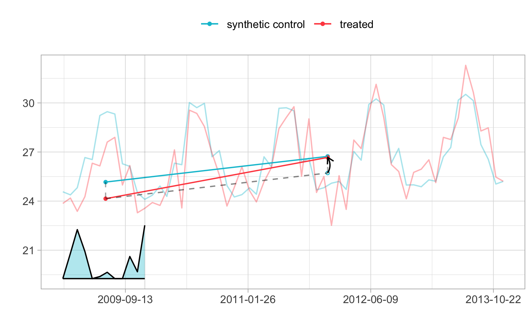
tau.hat <- synthdid_estimate(setup$Y, setup$N0, setup$T0)
se <- sqrt(vcov(tau.hat, method='placebo'))
sprintf('point estimate: %1.2f', tau.hat)
[1] "point estimate: 0.95"sprintf('95%% CI (%1.2f, %1.2f)', tau.hat - 1.96 * se, tau.hat + 1.96 * se)[1] "95% CI (0.10, 1.81)"plot(tau.hat)Assignment
Accept the Week 12 - Assignment and follow the same steps as last week and as described in the organization chapter.
Please also remember to fill out the course evaluation if you have not done so already.
For the following tasks, you should use the ride_12_multi.rds data.
The
synthdidpackages does not yet provide an implementation for staggered adoption. Build your own implementation that applies the estimator once for every adoption date and report the treatment effects.Find an appropriate measure that summarizes the treatment effects. Discuss in 1-2 sentences, what you think should be considered when constructing such a measure.
Report the short-term (1 year) and mid-term (3 years) treatment effects and compare them in an appropriate plot using the
ggplot2package.
