# A tibble: 6 × 9
  city    density employment   gdp population treated post  revenue period
  <chr>     <int>      <dbl> <dbl>      <dbl> <lgl>   <lgl>   <dbl> <date>
1 Atlanta     290      0.630  6.45       4.27 FALSE   FALSE    23.5 2003-01-01
2 Atlanta     290      0.630  6.45       4.27 FALSE   FALSE    24.3 2003-02-01
3 Atlanta     290      0.630  6.45       4.27 FALSE   FALSE    23.3 2003-03-01
4 Atlanta     290      0.630  6.45       4.27 FALSE   FALSE    27.7 2003-04-01
5 Atlanta     290      0.630  6.45       4.27 FALSE   FALSE    26.4 2003-05-01
6 Atlanta 290 0.630 6.45 4.27 FALSE FALSE 28.3 2003-06-0111 - Synthetic Control (1/2)
Slides & Recap
Over the past two weeks, we’ve explored how to use panel data to estimate causal effects with variations of the difference-in-differences estimator. This week, we’ll dive into another popular estimation technique: the synthetic control (SC) method. Originally designed for scenarios with very few treated units—often just one, like a single country—this method constructs a synthetic control unit by combining control units. This synthetic unit closely replicates the behavior of the treated unit before the intervention and acts as a counterfactual after the treatment. When the treated unit and the synthetic control unit align perfectly, we can relax the parallel trends assumption.
Practical example
Exploration
Consider the following example: you are working at a ride-sharing platform and you want to understand the effect of introducing a new feature on revenue, i.e. let’s say the introduction of self-driving cars. 1
Let’s directly take a look at the data.
As we approach the end of this module, I’ll be providing less guidance. Therefore, similar to last week, let’s dive into some data exploration.
Task 1: Answer the following questions:
- How many periods did we observe?
- How many units did we observe?
- How many units are in the treatment and how many are in the control group?
- What is the treatment period?
Code
# Exploration
# How many pre- and post periods?
T_pre <- n_distinct(ride[ride$post == 0, ]$period)
T_post <- n_distinct(ride[ride$post == 1, ]$period)

# How many units?
N1 <- n_distinct(ride[ride$treated == 1, ]$city)
N0 <- n_distinct(ride[ride$treated == 0, ]$city)

# What is first treatment period?
T0 <- min(ride[ride$post == 1, ]$period)

print(c(T_pre, T_post, N1, N0))
[1] 84 120 1 12Code
print(T0)[1] "2010-01-01"Task 2: Plot the revenue evolution over time.
Code
# Revenue over time
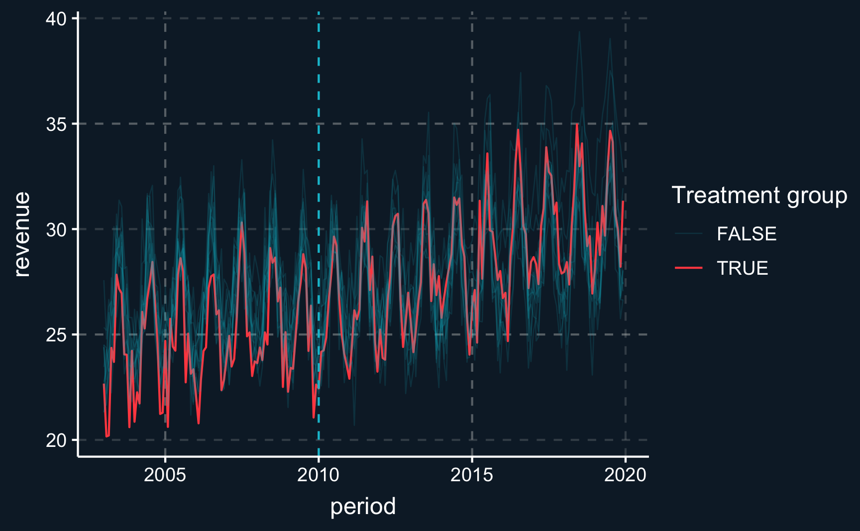
ggplot(
  ride,
  aes(
    x = period,
    y = revenue,
    group = city,
    color = factor(treated),
    linewidth = factor(treated)
  )) +
  geom_line(aes(alpha = factor(treated))) +
  geom_vline(xintercept = T0, linetype = "dashed") +
  scale_alpha_manual(values = c(.15, 1)) +
  scale_linewidth_manual(values = c(.3, .5)) +
  labs(color = "Treatment group", alpha = "Treatment group", linewidth = "Treatment group")
Task 3: Compare the treated city to the control cities in terms of the covariate and outcome distribution.
Code
# A tibble: 2 × 6
  treated density employment   gdp population revenue
  <lgl>     <dbl>      <dbl> <dbl>      <dbl>   <dbl>
1 FALSE      218.      0.641  6.14       2.54    27.6
2 TRUE       498.      0.608  6.36       9.43    27.0
Synthetic control
As we explore the synthetic control method, we’ll start by doing it manually. While you’ll most likely use pre-built packages in practice, performing the calculations by hand can provide a deeper understanding of the underlying mechanics of the method.
Here is a useful perspective to consider as we approach the data:
\[ \begin{equation} \left( \begin{array}{c|c} \begin{matrix} X_{11} & X_{12} & \cdots & X_{1T_0} \\ \hline X_{21} & X_{22} & \cdots & X_{2T_0} \\ \vdots & \vdots & \ddots & \vdots \\ X_{N1} & X_{N2} & \cdots & X_{NT_0} \end{matrix} & \begin{matrix} Y_{1T} \\ \hline Y_{2T} \\ \vdots \\ Y_{NT} \end{matrix} \end{array} \right) \equiv \left( \begin{array}{c|c} \begin{matrix} \mathbf{X}_{1} \\ \hline \mathbf{X}_{0} \\ \end{matrix} & \begin{matrix} Y_{1T} \\ \hline \mathbf{Y}_{0T} \\ \end{matrix} \end{array} \right) \end{equation} \]
We utilize the control units, often referred to as the “donor pool,” to replicate the pre-treatment observations of the treated unit. For each control unit, we assign a weight, which is then used to impute the counterfactual outcome for the treated unit. Specifically, \(Y_{1T_t}(0)\) is imputed using a weighted average of \(\mathbf{Y}_{0T_t}\).
For our initial step, we’ll focus solely on pre-treatment outcomes, setting aside covariates for now. Our goal is to accurately reproduce the pre-treatment outcome of the treated unit by adjusting the weights assigned to the pre-treatment outcomes of the control units.
Let’s begin by organizing our data into four distinct blocks:
- Pre-treatment control \(\mathbf{X}_{0}\)
- Pre-treatment treated \(\mathbf{X}_{1}\)
- Post-treatment control \(Y_{0T}\)
- Post-treatment treated \(Y_{1T}\)
Initially, we’ll focus on revenue as our primary outcome variable and introduce covariates later in the analysis to refine our model.
Task 4: Split the data and extract the four blocks.
Code
# Split and extract 4 matrices
y0_pre <- ride |>
  filter(post == 0, treated == 0) |>
  pivot_wider(id_cols = "period", names_from = "city", values_from = "revenue") |>
  select(-period) |>
  as.matrix()

y1_pre <- ride |>
  filter(post == 0, treated == 1) |>
  pivot_wider(id_cols = "period", names_from = "city", values_from = "revenue") |>
  select(-period) |>
  as.matrix()

y0_post <- ride |>
  filter(post == 1, treated == 0) |>
  pivot_wider(id_cols = "period", names_from = "city", values_from = "revenue") |>
  select(-period) |>
  as.matrix()

y1_post <- ride |>
  filter(post == 1, treated == 1) |>
  pivot_wider(id_cols = "period", names_from = "city", values_from = "revenue") |>
  select(-period) |>
  as.matrix()

# Print "donor pool"
print(head(y0_pre))
Atlanta Columbus Davidson Indianapolis Jackson Jacksonville Memphis Orange Pittsburgh San Diego San Francisco St. Louis
[1,] 23 25 28 25 22 21 22 24 21 24 25 23
[2,] 24 24 25 23 24 22 24 22 22 22 25 23
[3,] 23 23 26 26 26 23 24 24 23 23 27 24
[4,] 28 26 27 25 27 24 25 26 22 24 26 25
[5,] 26 29 30 26 25 26 26 27 24 25 26 26
[6,] 28 29 29 30 29 26 27 29 25 29 31 30Horizontal regression
To find the synthetic control weights, \(\mathbf{W}* = (w_2^*, \ldots, w_{N+1}^*)\) that minimizes \(\| \mathbf{X}_1 - \mathbf{X}_0 \mathbf{W} \|\), a simple way is to run an ordinary linear regression. At first, it might be a bit confusing, but, prior to the treatment, we can regress the treated unit on the control units and see which control units can explain the treated unit best. You just need two of the blocks you just created.
Task 5: Run the linear regression and print the obtained weights. What is an observation in this setup? What is the meaning of the coefficients?
Code
# Weights from OLS
ols <- lm(y1_pre ~ 0 + y0_pre)
w_ols <- coef(ols)

print(as.data.frame(w_ols) |> arrange(-w_ols))
w_ols
y0_preSan Francisco 0.2766
y0_preSt. Louis 0.2322
y0_preAtlanta 0.2236
y0_preMemphis 0.1639
y0_preOrange 0.1452
y0_preJackson 0.1334
y0_prePittsburgh 0.0590
y0_preJacksonville 0.0410
y0_preDavidson 0.0064
y0_preColumbus -0.0881
y0_preSan Diego -0.1183
y0_preIndianapolis -0.1408Having obtained the weights, we can now proceed to calculate the estimate that we are ultimately interested in, the \(ATT\). For the periods following the treatment, we subtract the synthetic outcome from the observed outcome for the treated unit:
\[ \hat{\tau}_{1t} = Y_{1t} - \sum_{i=2}^{N+1} w_i^* Y_{it} \quad \forall \quad t > T_0 \]
This expression yields the treatment effect per period. By averaging across the treatment periods, you retrieve the \(ATT\).
Matrix multiplication with %*% in R performs a dot product of rows and columns, where each element of the resulting matrix is the sum of the products of corresponding elements from the rows of the first matrix and the columns of the second matrix. This operation requires that the number of columns in the first matrix matches the number of rows in the second matrix.
Task 6: Calculate the ATT.
Code
[1] 1.6Task 7: Calculate the pseudo-ATT before the treatment takes place. What value do you expect?
Code
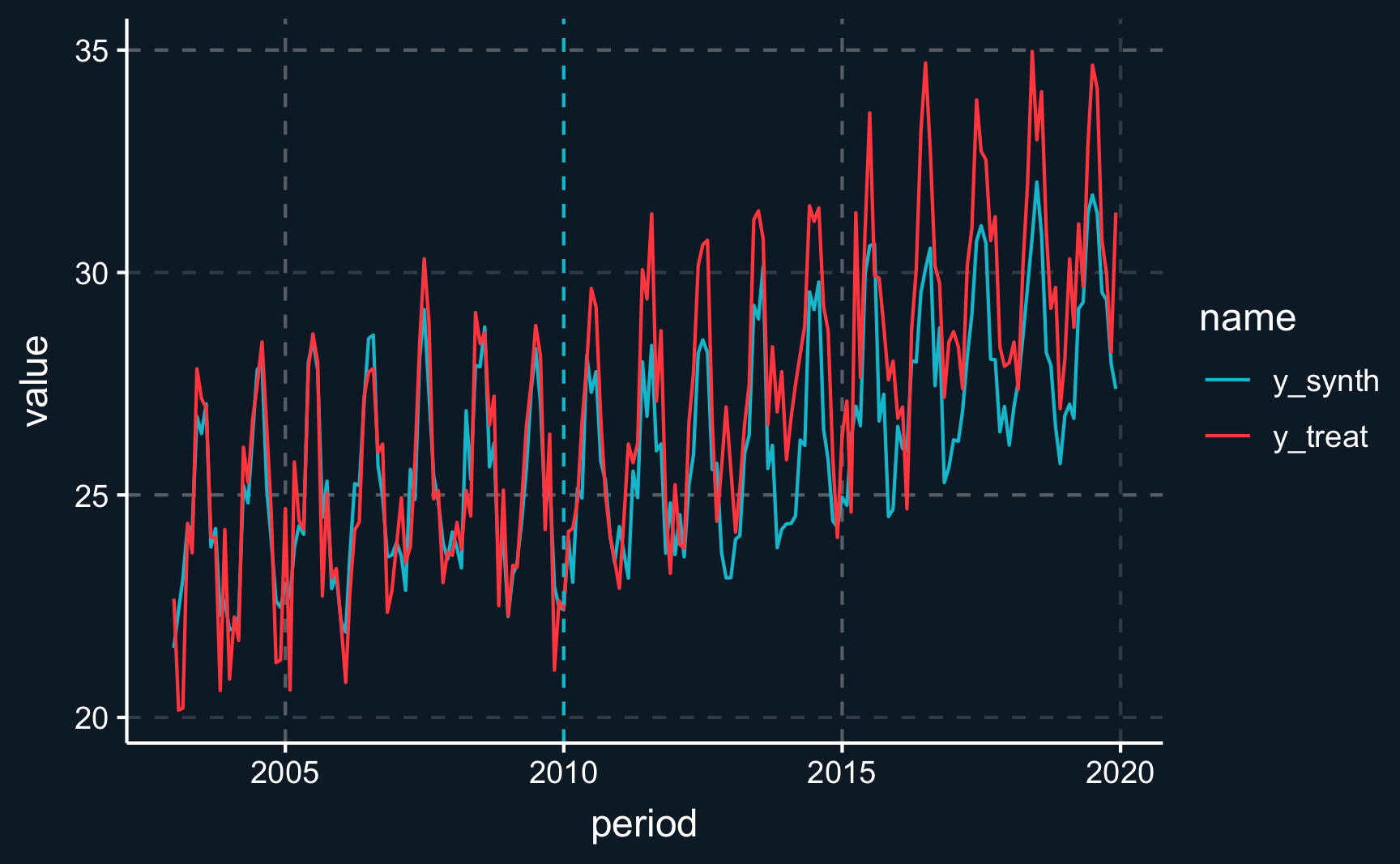
[1] -0.019Let’s plot the synthetic and observed unit.
# Create data frame with synthetic control and treated unit
sc_vs_trt <- tibble(
  period = unique(ride$period),
  y_synth = c(y_sc_pre, y_sc_post),
  y_treat = c(y1_pre, y1_post)
) |>
  pivot_longer(cols = c("y_synth", "y_treat"))

# Line plot with treatment date highlighted
ggplot(sc_vs_trt, aes(x = period, y = value, group = name, color = name)) +
  geom_line() +
  geom_vline(xintercept = T0, linetype = "dashed")
Because we will want to plot in the subsequent steps as well, let’s create a function that helps us avoiding to rewrite the code. The only thing that is variable in these lines of codes is the estimated synthetic control unit. Check for yourself that you can reproduce the previous plot using the function.
# Generate plot of synthetic unit and observed treated unit
plot_synth <- function(y_sc_pre, y_sc_post) {
  # Data to plot
  sc_vs_trt <- tibble(
    period = unique(ride$period), # periods (will be replicated)
    y_synth = c(y_sc_pre, y_sc_post), # synthetic outcomes
    y_treat = c(y1_pre, y1_post) # observed outcomes of treated unit
  ) |>
    # long format for ggplot
    pivot_longer(cols = c("y_synth", "y_treat"))

  ggplot(sc_vs_trt,
         aes(
           x = period,
           y = value,
           group = name,
           color = name)
         ) +
    geom_line() +
    geom_vline(xintercept = T0, linetype = "dashed")
}
Period weights
We have successfully replicated the pre-treatment outcomes quite closely. In doing so, we’ve implicitly assumed that each period leading up to the treatment carries equal significance for our analysis. However, it’s reasonable to consider that more recent periods might be more indicative of the trends following the treatment. To accommodate this insight, we can simply adjust our methodology to place greater emphasis on these more recent periods. This minor modification will help refine our approach and potentially yield more accurate predictions.
\[ \begin{aligned} \mathbf{W}^* = \arg\min_{\mathbf{W}} \| \sqrt{V}\mathbf{X}_1 - \mathbf{X}_0 \mathbf{W} \|_2^2 &= \arg\min_{\mathbf{W}} [(\mathbf{X}_1 - \mathbf{X}_0 \mathbf{W})' \mathbf{V} (\mathbf{X}_1 - \mathbf{X}_0 \mathbf{W})] \\ &= \arg\min_{\mathbf{W}} \sum_{m=1}^{k} v_m \bigg( X_{1m} - \sum_{i=2}^{N+1} w_iX_{im}\bigg)^2 \\ \end{aligned} \]
The sweep() function in R applies an operation (such as addition, subtraction, multiplication, or division) to the rows or columns of a matrix or array, using a corresponding vector of values, effectively “sweeping” the operation across the specified margin (rows or columns) of the data. In R, the margin 1 and 2 refer to rows and columns, respectively.
First, we just replicate the previous estimate by having uniform weights (each period receives weight = 1).
# Including weights with uniform weights
a_uni <- rep(1, T_pre)
y0_pre_uni <- sweep(y0_pre, 1, a_uni, "*")
y1_pre_uni <- sweep(y1_pre, 1, a_uni, "*")

ols_uni <- lm(y1_pre_uni ~ 0 + y0_pre_uni)

# Check for equality
all(coef(ols) == coef(ols_uni))
[1] TRUEFor now, we’ll pause here and move to the next section. But you will need period weights for your assignment.
Weight constraints
So far, we have not taken into account that, as discussed in the lecture, weights are subject to two conditions:
\(\mathbf{W} = (w_2, \ldots, w_{N+1})'\), with \(w_i \geq 0\) and \(\sum_{i=2}^{N+1} w_i = 1\).
However, the sum of weights from before are:
# Sum of weights
sum(w_ols)
[1] 0.93For optimization subject to constraints, we need to install and load CVXR, a package of convex optimization. Defining the objective and the constraint, we can solve for the optimal weights \(w\) for the synthetic control unit.
Let’s check whether the weights fulfill the constraints.
# Check constraints
sum(w_star)
[1] 1sum(w_star >= 0)[1] 4round(w_star, 2) [1] 0.00 0.00 0.00 0.00 0.00 0.24 0.10 0.21 0.45 0.00 0.00 0.00# A tibble: 12 × 2
city `round(w_star, 2)`
<chr> <dbl>
1 Atlanta 0
2 Columbus 0
3 Davidson 0
4 Indianapolis 0
5 Jackson 0
6 Jacksonville 0.24
7 Memphis 0.1
8 Orange 0.21
9 Pittsburgh 0.45
10 San Diego 0
11 San Francisco 0
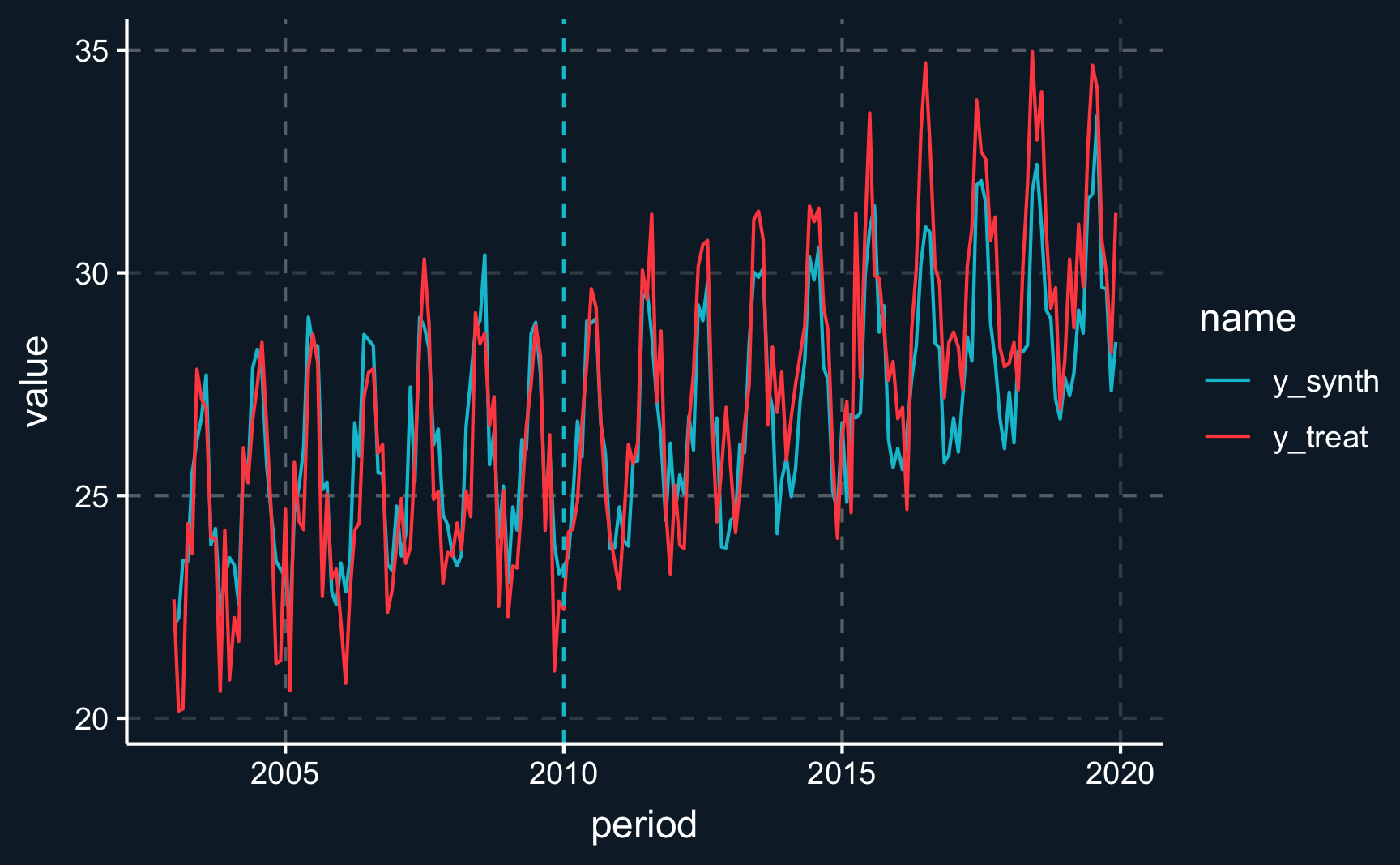
12 St. Louis 0 Task 8: Plot the treated unit and synthetic control prior to and after the treatment.
Assignment
Accept the Week 11 - Assignment and follow the same steps as last week and as described in the organization chapter.
Please also remember to fill out the course evaluation if you have not done so already.
In 3-4 sentences, compare the assumptions required for difference-in-differences and synthetic control.
Argue why in this scenario, you cannot run an A/B test at the ride-level and are better of with the synthetic control method.
Combine what you have learned about the constrained minimization and weighting of periods and compute the \(ATT\) by giving higher weight to more recent periods (please make sure that the sum of the period weights is equal to the number of periods: usually each period would have weight 1). Additionally, plot the data.
-
So far, we have not done any inference. A simple measure of the confidence we have in our estimate can be obtained by repeating the estimation procedure but swapping out the treated city. This way we obtain a “pseudo” treatment effect \(ATT_{pseudo}\) for each city and to reject the hypothesis of no treatment effect for our actually treated unit, the \(ATT\) should be larger than most of the other “pseudo” treatment effects \(ATT_{pseudo}\).
Perform this so called permutation test and report the percentage (“p-value”) of larger “pseudo” treatment effects.
Plot the effects for all cities and highlight the actually treated city graphically.
Footnotes
Inspired by: https://matteocourthoud.github.io/post/synth/↩︎


