# Instrumental Variable Estimation - Application
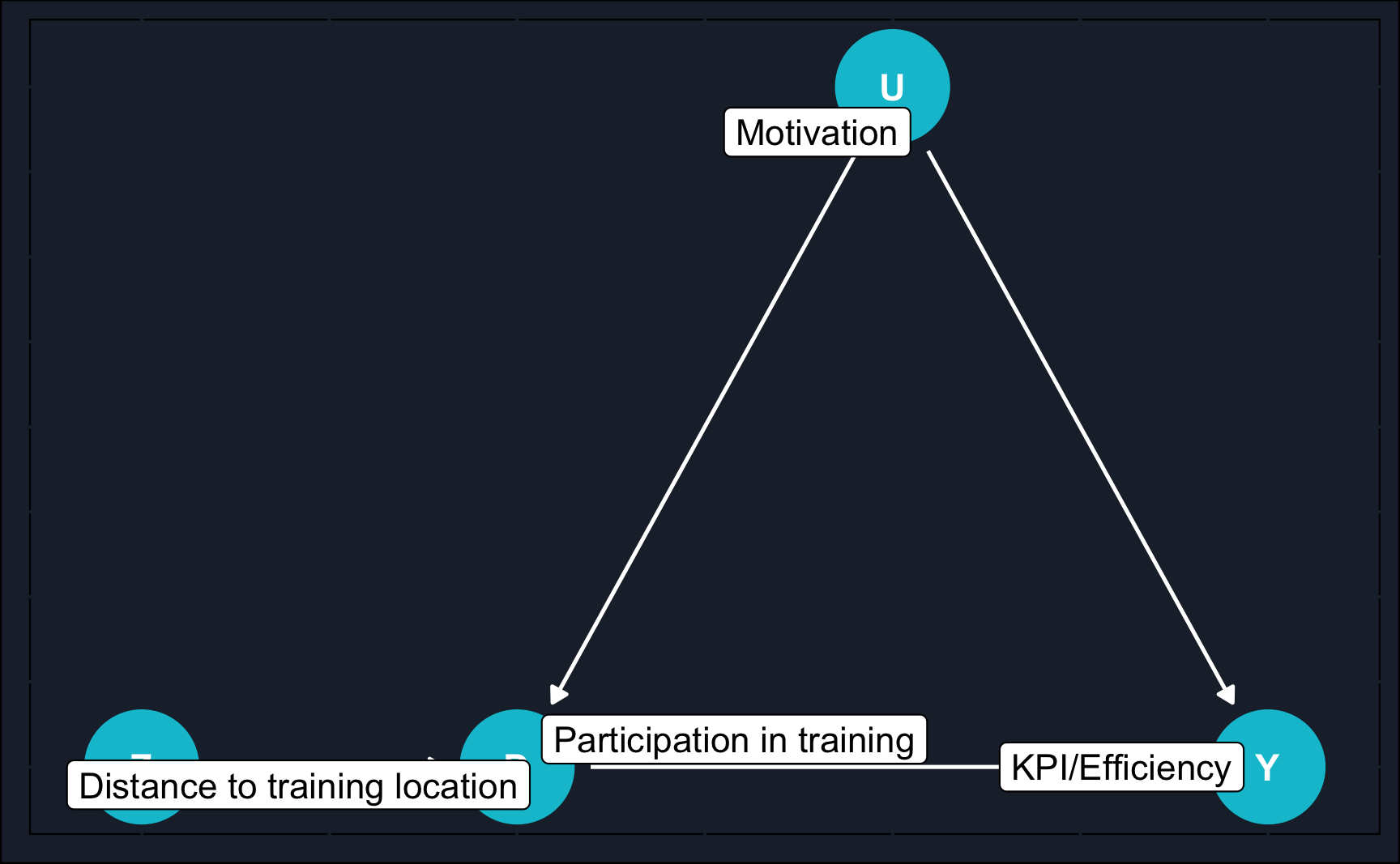
iv_expl <- dagify(
  Y ~ D,
  Y ~ U,
  D ~ U,
  D ~ Z,
  exposure = "D",
  latent = "U",
  outcome = "Y",
  coords = list(x = c(U = 1, D = 0, Y = 2, Z = -1),
                y = c(U = 1, D = 0, Y = 0, Z = 0)),
  labels = c("D" = "Participation in training",
             "Y" = "KPI/Efficiency",
             "U" = "Motivation",
             "Z" = "Distance to training location")
)
ggdag(iv_expl, text = T) +
  guides(color = "none") +
  theme_dag_cds() +
  geom_dag_point(color = ggthemr::swatch()[2]) +
  geom_dag_text(color = "white") +
  geom_dag_edges(edge_color = "white") +
geom_dag_label_repel(aes(label = label))Instrumental Variables
Introduction
The method we introduce in this chapter is called instrumental variables estimation (IV), a quasi-experimental method heavily used in economics to identify causal effects in observational studies with unobserved confounders. Thus, it can control for omitted variable bias which is present when we were either not able to collect all relevant data or we are not aware of some confounders.
Due to not observing particular confounders, we cannot close the backdoor path by for example matching or regression. IV provides an alternative by introducing an additional variable (the instrumental variable/instrument), which affects the outcome only through the treatment variable.
The instrumental variable is exogenous, i.e. there is no other variable in the model influencing the value of the instrument (no arrow pointing to the instrument). Thus, it mimics an experiment by exploiting the exogenous variation in treatment due to the instrument. Endogenous variation from unobserved confounders can be disregarded as we are only considering the variation in treatment caused by the instrument.
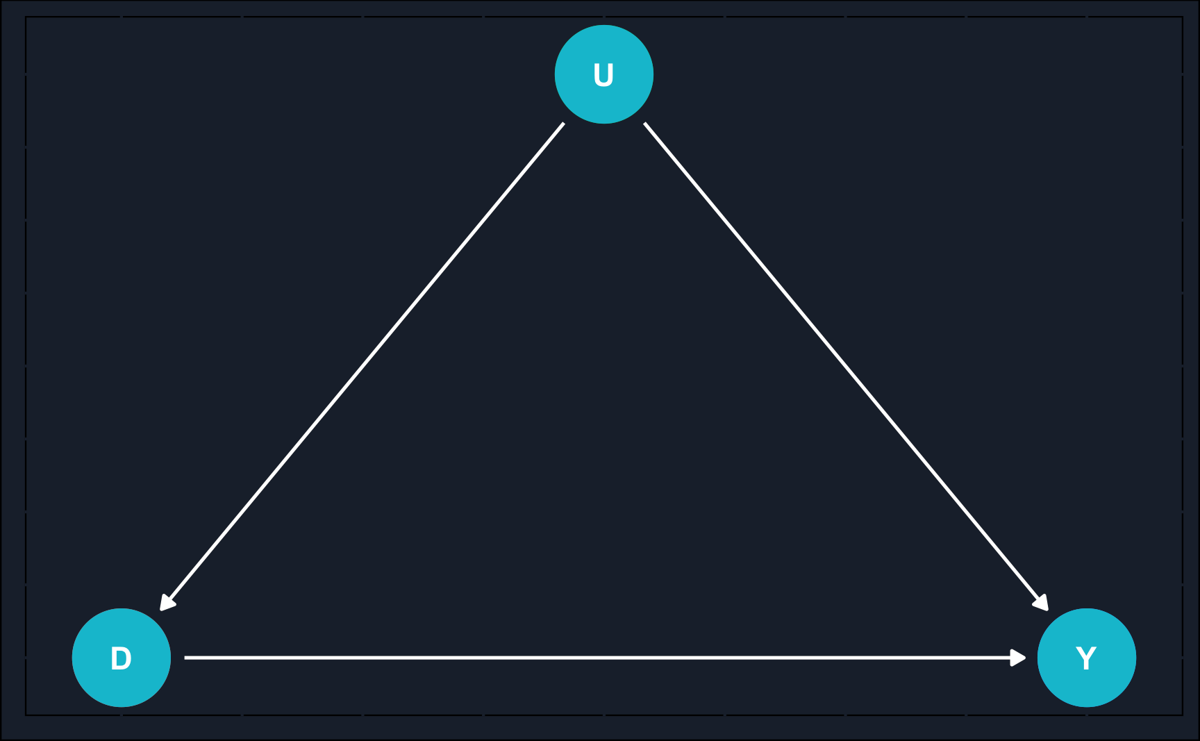
IV can be illustrated using DAGs. On the left, there is a potential initial situation you could find yourself in: you want to examine the effect of \(D\) on \(Y\), but unfortunately, there is an unobserved confounder (=omitted variable) that you would have to adjust for to identify the direct effect. As \(U\) is unobserved, there is no way to close the backdoor path by methods like matching, regression etc. This is where IV comes to rescue.
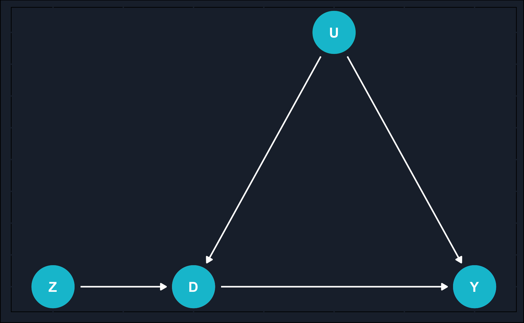
As you can see on the right, now \(D\) mediates between an instrument \(Z\) and outcome \(Y\). There is no direct path between \(Z\) and \(Y\) and therefore \(Z\) affects \(Y\) only through \(D\). For the instrument validity, there are a few assumptions that need to be fulfilled, which we discuss later in detail but summarizing, we need
Relevance: \(Z \rightarrow D, \,\,\, Cor(Z,D) \neq 0\) [testable]. The instrument \(Z\) needs to have an impact on the treatment \(D\).
Excludability: \(Z \rightarrow D \rightarrow Y,\,\, Z \not\to Y, \,\,\, Cor(Z, Y|D) =0\) [partly testable]. The instrument \(Z\) influences the outcome \(Y\) only through the treatment variable \(D\).
Exogeneity: \(U \not\to Z, \,\,\, Cor(Z, U)=0\) [not testable]. The unobserved confounder \(U\) is uncorrelated with the instrument \(Z\).
Application
To delve deeply into the requirements and provide a detailed explanation of how to estimate the effects, let’s take an example for illustration.
Let us imagine the following situation. You are manager of a company that allows its workers to work remotely from any location. Now you want to implement a voluntary training program to improve the skills of your workforce. Other than the general work, training programs are held in a number of locations on-site. To measure the effect of your training program on a worker’s output, you are able to collect
- \(D\): whether an individual worker has participated in the training program
- \(Y\): his/her work output (something like a key performance indicator (KPI))
If we can assume treatment is not determined by unobserved confounders variables, estimating a causal effect is possible. That means, that no other unmeasured variable confounds the relationship between treatment and outcome.
A major factor \(U\) influencing both treatment \(D\) and outcome \(Y\) could be motivation as more more motivated workers are more likely to participate in a training program to improve their skills and also more likely to be more productive. Unfortunately, motivation is variable that is very hard to measure. Workers with a low level of motivation will try to hide it while workers with a high level of motivation might not be able to show it.
Therefore, motivation \(U\) opens a backdoor path between \(D\) (= program participation) and \(Y\) (worker output) which cannot be closed. To eliminate the bias caused by an omitted variable, the strategy is to use an instrument.
We can exploit the fact that the distance to training location is known. At first glance, distance could serve as an instrument \(Z\) as it related to \(D\) (close distance to training location might increase participation likelihood) and is not otherwise related to outcome \(Y\).
To establish the validity of an instrument, five prerequisites must be satisfied:
Stable unit treatment value assumption: Potential outcomes for a unit do not vary with treatments assigned to other units. Note that it does not mean that treatment assignment is independent across units. For example, if a worker participates in training because his/her colleague does so, it is not a violation of the assumption. A violation only occurs when the participation of a colleague affects one’s own outcome.
Independence assumption: There is no confounding between instrument \(Z\) and treatment \(D\) and also no confounding between \(Z\) and outcome \(Y\). In our application, it means there is no factor that both influences the proximity to the closest training location and program participation or worker efficiency. If we want to think of a potential violation, we could imagine more motivated workers living closer to a training location (e.g. if the headquarter is a training location) and thus, there would be confounding between \(Z\) and both treatment assignment and outcome.
Exclusion restriction: As already mentioned above, the instrument does not directly affect outcome, but only through the treatment. Other than the consideration in 2), there is no obvious reason why living closer or further away from a training location would affect an individual worker’s efficiency. Please note that this assumption is not testable.
Instrument relevance: There should be a correlation of \(Z\) and \(D\). The stronger the association, the more powerful an instrument is. We will later check the correlation between both variables (in the so called “first stage”).
Monotonicity assumption: Instrument (weakly) operates in same direction, i.e. it might be the case, that the instrument does not affect all units, but for all units that are affected the effect goes in the same direction.
Using the framework below, monotonicity is satisfied, if there are no defiers. Let’s define what defiers are. In general, there are four types of observation units with regard to their value of \(Z\) and \(D\).
Compliers: \(D\) is affected by \(Z\) in “correct” direction.
Defiers: \(D\) is affected by \(Z\) in “wrong” direction.
Never takers: \(D = 0\) in all cases, regardless of \(Z\).
Always takers: \(D = 1\) in all cases, regardless of \(Z\).
If all of the assumptions are satisfied, we are able to estimate the average treatment effect for compliers, which is also known as local average treatment effect (\(LATE\)). With regard to our application, we estimate the average treatment effect only for individuals whose decision to participate was affected by the their distance to the training location.
Exploration
For the sake of explanation, we generate a synthetic data set with the variables \(Z\), \(D\) and \(Y\) as defined above. We also include the unobserved variable \(U\). This way, we can better explain where the bias comes from and how it affects the estimated treatment effect. The true treatment effect, which is the direct effect of \(D\) on \(Y\), is set to \(1\). We also add some random noise, so relationships are not perfect and what you will see is closer to reality.
# Show data
df
From the table, you already have an idea what the data structure and types look like. But when developing our analysis strategy, we are mainly interested in relationships between the variables, so let’s have a look at the correlation matrix. It is a first step in assesing certain prerequisites for a valid IV strategy. Please also note, that we include \(U\) here, but in general, you do not observe \(U\), which was the reason why we need to use IV in the first place. It is just for the purpose of explanation that we include it here.
           distance program motivation   kpi
distance       1.00   -0.56       0.01 -0.47
program       -0.56    1.00       0.39  0.92
motivation     0.01    0.39       1.00  0.55
kpi           -0.47    0.92       0.55  1.00
From the correlation matrix, we can take a few important insights. There is a significant negative correlation between distance and program participation, which is also called first-stage and confirms the relevance of our instrument. The distance to the next training location does affect decision to participate in a training. This is assumption (4) from above.
Having a synthetic data set, we can also see that our instrument is uncorrelated with the unobserved variable motivation, which means there is no confounding as stated in assumption (2). Usually, however, we would not be able to test this assumption due to an unobservable variable not being observed. Moreover, there could be additional confounders. With merely statistical concepts, we cannot prove that the effect of \(Z\) on \(Y\) goes only through \(D\). We have to argue why that is the case.
Corresponding to our DAG, we also see that both program participation and KPI are correlated with the (unobserved) motivation, which thus opens another path between treatment and outcome. Being unable to close this path, we actually need an instrument in this situation.
Additionally to relying on a correlation matrix, it could be very useful to also plot the data to check relationships between variables.
Modeling
Confounding
When you plausibly argue that your instrument is valid, you would usually perform 2SLS, short for Two Stage Least Squares. We’ll come to that shortly, but because we have all the data, we can also check what the bias would be in case we would not use an instrument and ignore the confounder.
Remember, the true treatment effect is 1 in this case. Therefore, when we regress \(Y\) on \(D\) and \(U\), we should be able to recover this effect. And when you look at the regression output, in fact, we do. It is not exactly equal 1, but that is due to sampling noise.
# First of all, let's look at the coefficients of the "full" (but unobservable)
# model. It is unobservable, as it includes motivation, which in reality is
# a variable that is very hard to collect or measure.
# Coefficients are expected to be close to what he have defined in the data
# generation section.
model_full <- lm(kpi ~ program + motivation, data = df)
summary(model_full)
Call:
lm(formula = kpi ~ program + motivation, data = df)

Residuals:
    Min      1Q  Median      3Q     Max
-0.7095 -0.1358 -0.0016  0.1359  0.7078

Coefficients:
            Estimate Std. Error t value Pr(>|t|)
(Intercept) -0.01391    0.01124   -1.24     0.22
program      1.00969    0.00563  179.32   <2e-16 ***
motivation   1.02004    0.02156   47.31   <2e-16 ***
---
Signif. codes:  0 '***' 0.001 '**' 0.01 '*' 0.05 '.' 0.1 ' ' 1

Residual standard error: 0.2 on 5997 degrees of freedom
Multiple R-squared:  0.89,  Adjusted R-squared:  0.89
F-statistic: 2.43e+04 on 2 and 5997 DF,  p-value: <2e-16
But what would happen if we ignored the confounder \(U\) (motivation) and only regress \(Y\) (KPI/efficiency) on \(D\) (program participation)? We do not close the backdoor path and consequently, the effect is overestimated.
We can see that the coefficient for program participation is higher than expected, i.e. it has an upward bias. This is because, it takes some of the variation that is actually attributable to motivation into the coefficient of program participation. More motivatd employees are more likely to participate in the program and have higher outcomes even without participation. This confirms the need to include an instrument to model causal effects when there is no way to include the confounder.
# Modeling the data without the unobservable variable, i.e. only including
# program participation in this case, returns a biased coefficient as the
# relationship between program and the outcome is biased by a collider.
model_biased <- lm(kpi ~ program, data = df)
summary(model_biased)
Call:
lm(formula = kpi ~ program, data = df)

Residuals:
    Min      1Q  Median      3Q     Max
-0.8203 -0.1604 -0.0018  0.1599  0.8175

Coefficients:
            Estimate Std. Error t value Pr(>|t|)
(Intercept)  0.48878    0.00429     114   <2e-16 ***
program      1.11462    0.00606     184   <2e-16 ***
---
Signif. codes:  0 '***' 0.001 '**' 0.01 '*' 0.05 '.' 0.1 ' ' 1

Residual standard error: 0.23 on 5998 degrees of freedom
Multiple R-squared:  0.849, Adjusted R-squared:  0.849
F-statistic: 3.38e+04 on 1 and 5998 DF,  p-value: <2e-16
2SLS
Two Stage Least Square is the estimation technique for IV and consists, as it names suggest, of two stages. In the first stage, the treatment variable is regressed on the instrument and in the second stage, the estimated values of the first stage are used as a regressors for the outcome. It sounds a little bit confusing, so let’s write it down. Remember, \(D\) is our treatment, \(Z\) the instrument and \(Y\) the outcome.
First stage:
\[ D_i = \gamma_0 + \gamma_1Z_i + \nu_i \]
Second stage:
\[ Y_i = \beta_0 +\beta_1\widehat{D_i} +\epsilon_i \]
Lower cases indicate single observations, so \(i\) indicates for example the row in our data set. What is important to note, is that in the second stage, we do not use \(D_i\), but instead \(\widehat{D_i}\). The hat indicates that these are fitted values from the first stage.
We can do 2SLS manually in R, but for reasons I will get to later, it is recommended to use libraries built to run 2SLS. However, for purpose of explanation, we’ll do it also manually here.
First stage: As already discussed, regress treatment variable on instrument and obtain the fitted model. The model coefficient returned by the model summary should be significant, otherwise there is reason to doubt the relevance and validity of the instrument. You can also look at the F-statistic, which should be above 10.
Although program is a binary variable, we use linear regression instead of logistic regression. Otherwise, 2SLS does not provide correct results. A linear regression predicting binary outcomes is called linear probability model (LPM).
Here, the instrument is highly significant. The higher the distance, the lower the likelihood of participation.
Call:
lm(formula = program ~ distance, data = df)

Residuals:
    Min      1Q  Median      3Q     Max
-1.1268 -0.3320 -0.0371  0.3479  1.0206

Coefficients:
            Estimate Std. Error t value Pr(>|t|)
(Intercept)   1.4680     0.0191    76.8   <2e-16 ***
distance     -1.6207     0.0307   -52.7   <2e-16 ***
---
Signif. codes:  0 '***' 0.001 '**' 0.01 '*' 0.05 '.' 0.1 ' ' 1

Residual standard error: 0.41 on 5998 degrees of freedom
Multiple R-squared:  0.317, Adjusted R-squared:  0.316
F-statistic: 2.78e+03 on 1 and 5998 DF,  p-value: <2e-16
Let’s look at the fitted values from the first stage. The fitted values is what you get when you use the calculated coefficients and for each observation compute what the model predicts as an expected value. So, they are most likely a different from the actual values. How different they are depends on the goodness of fit of your model. This is why it is important that your instrument has a good explanatory value for the treatment variable.
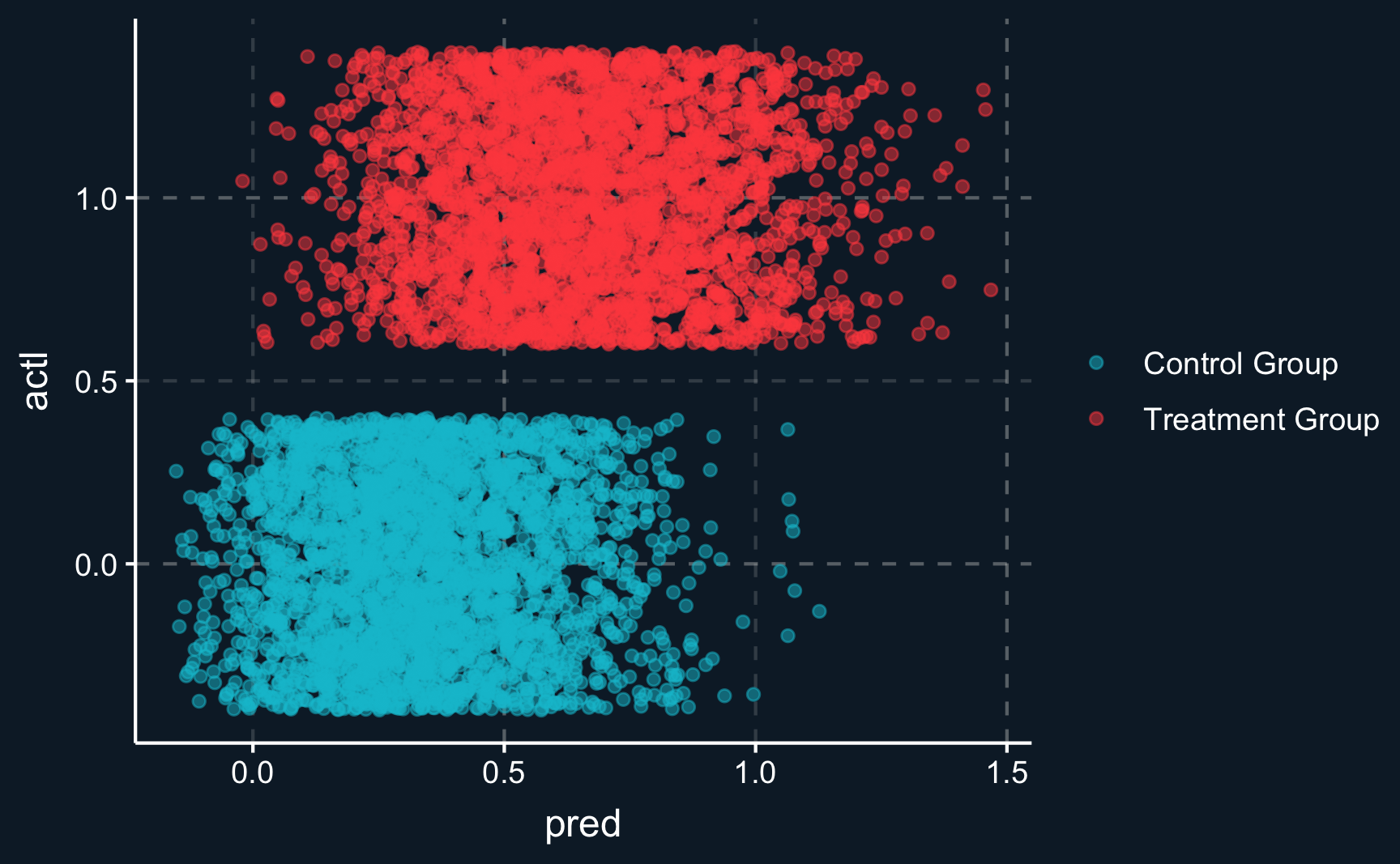
Let’s see how well we can explain the decision to participate using the distance to the training location. For employees that actually participated, predicted probabilities are on average higher than for those who have not participated. However, there is a large amount of overlap between both groups. By the way, because we used a linear probability model, not all probabilities are between 0 and 1.
# Predicted 'probabilities' from first stage
pred_fs <- predict(first_stage)

# Create table with predictions and actual decisions
pred_vs_actl <- tibble(
  pred = pred_fs,
  actl = df$program
)

# Plot predictions vs original
ggplot(pred_vs_actl, aes(x = pred, y = actl, color = as.factor(actl))) +
  geom_jitter(alpha = .5) +
  scale_color_discrete(labels = c("Control Group", "Treatment Group")) +
theme(legend.title = element_blank())Now we continue to use the fitted values from the first stage and plug it in the second stage to get the local average treatment effect. We see that the coefficient for the effect is close to one as constructed and we were able to eliminate the omitted variable bias.
Call:
lm(formula = df$kpi ~ first_stage$fitted.values)

Residuals:
    Min      1Q  Median      3Q     Max
-1.5789 -0.4053 -0.0111  0.4063  1.7100

Coefficients:
                          Estimate Std. Error t value Pr(>|t|)
(Intercept)                 0.5423     0.0141    38.5   <2e-16 ***
first_stage$fitted.values   1.0076     0.0245    41.1   <2e-16 ***
---
Signif. codes:  0 '***' 0.001 '**' 0.01 '*' 0.05 '.' 0.1 ' ' 1

Residual standard error: 0.53 on 5998 degrees of freedom
Multiple R-squared:  0.22,  Adjusted R-squared:  0.22
F-statistic: 1.69e+03 on 1 and 5998 DF,  p-value: <2e-16
However, it is recommended to use functions, like e.g. iv_robust() from the estimatr package, as it yields correct standard errors. You see that the coefficient is the same but the standard errors slightly differ.
# Using our instrument (distance to training location), we try to eliminate the
# bias induced by the omitted variable. If all assumptions regarding the validity
# of our instrument are met, the resulting coefficient should be
# close to what we have defined above.
library(estimatr)
model_iv <- iv_robust(kpi ~ program | distance, data = df)
summary(model_iv)
Call:
iv_robust(formula = kpi ~ program | distance, data = df)

Standard error type:  HC2

Coefficients:
            Estimate Std. Error t value Pr(>|t|) CI Lower CI Upper   DF
(Intercept)    0.542    0.00639    84.9        0    0.530    0.555 5998
program        1.008    0.01126    89.5        0    0.986    1.030 5998

Multiple R-squared:  0.841 ,    Adjusted R-squared:  0.841
F-statistic: 8.01e+03 on 1 and 5998 DF,  p-value: <2e-16
Conclusion
IV is an extremely popular research design but you have to be very careful when using it - particularly due to the fact that some of the necessary assumptions are untestable. This is why it is essential to have knowledge about the studied phenomenon to convincingly argue why the research design is valid and assumptions are plausible.
Moreover you have to question yourself, whether you measure the effect you are actually interested in. As you only measure the effect for compliers, for people who are affected by the instrument, the treatment effect is a local average treatment effect (LATE). And in case of heterogeneous treatment effects across the whole population, the LATE is different from the ATE.
Assignment
Imagine the following situation: you have developed an app and you are already having an active user base. Of course, some users are more active than other users. Also, users might use the app for different purposes. In general, user behavior likely depends on a lot of unobserved characteristics.
Obviously, your goal is to keep users as long as possible on the app to maximize your ad revenues. To do that, you want to introduce a new feature and see how it affects time spent on the app. Simply comparing users who use the newly introduced feature to users who don’t would result in a biased estimate due to the unobserved confounders regarding their activity and willingness to use a new feature.
Therefore, you perform a so called randomized encouragement trial, where for a random selection of users, a popup appears when opening the app and encourages these users to test new feature. The users who are not randomly selected don’t get a popup message but could also use the new feature.
After a while you collect data on users’ activity and also if they were encouraged and if they used the new feature. To see the data, load rand_enc.rds. Do the following steps:
Draw a DAG of how you understand the relationships.
Compute the naive, biased estimate.
For the assumptions that can be (partly) tested, check whether they are satisfied by either computing correlations or drawing plots. Argue whether instrumental variable estimation is an adequate procedure.
Compute the IV estimate using 2SLS and compare it to the naive estimate. Would you consider the naive estimate biased, and if yes, does it have an upward or downward bias?
Please see here how you have to successfully submit your solutions. I would recommend you to solve the assignments first in .R scripts and in the end convert them to the required format as explained in the submission instructions.


