Matching and Subclassification

Published

October 16, 2023

Problem

Almost always, the problem we are trying to solve in causal inference relates to the fundamental problem of causal inference, the fact that we cannot observe two states for one particular observation unit, e.g. we cannot see how a person’s health status after taking a specific drug and after not taking the same drug. Consequently, we cannot know the individual treatment effect.

Thus, we said we can make use of averages and try to estimate the average treatment effect by taking the difference between a group of treated observation units and a group of untreated observation units. Written in a formula, we can present it as

\[ ATE = E[Y_1| D = 1] - E[Y_0 | D = 0] \]

Assuming that individuals (or other kinds of observation units) were randomly assigned for example to take the drug, then this result gives us exactly what we want. It compares the outcomes of groups under treatment with groups not under treatment (control).

But the estimate hinges on the assumption that both groups are comparable, formally

\[ E[Y_0|D=0] = E[Y_0|D=1] \]

which we cannot test but in randomized settings we have good reason to believe it to be true. Under these circumstances, average treatment effect ($ATE$) and the average treatment effect on the treated ($ATT$) are equal.

However, if there are underlying group differences because the treatment assignment was not randomized and e.g. individuals were able to choose their treatment, we are not measuring the estimate that we are interested in. Then, the difference between $ATE$ and $ATT$ is what we call selection bias, an unmeasured factor representing systematic bias:

\[ ATE = ATT + \text{selection bias} \]

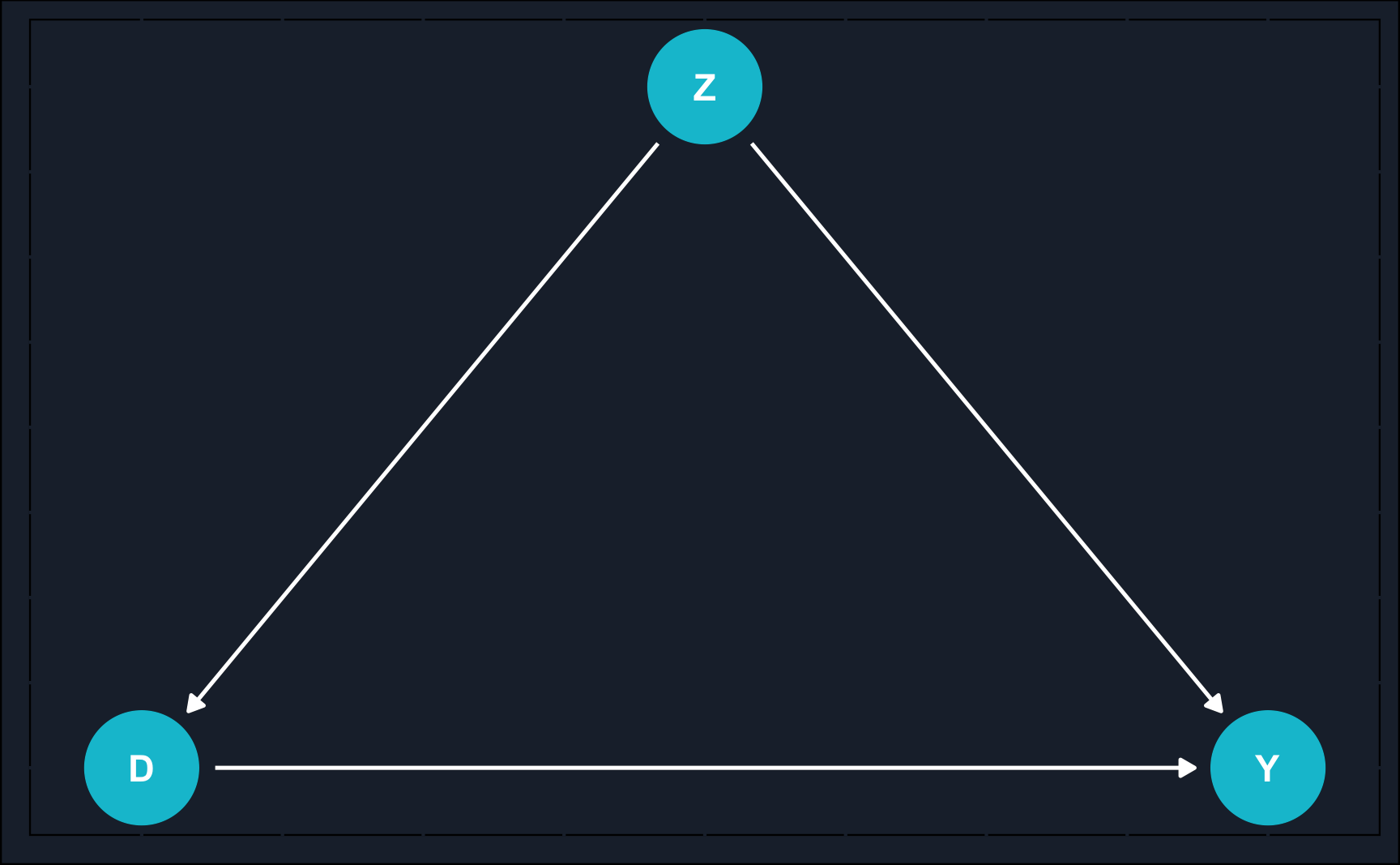
Graphically, we can show an example of when the naive estimate would fail.

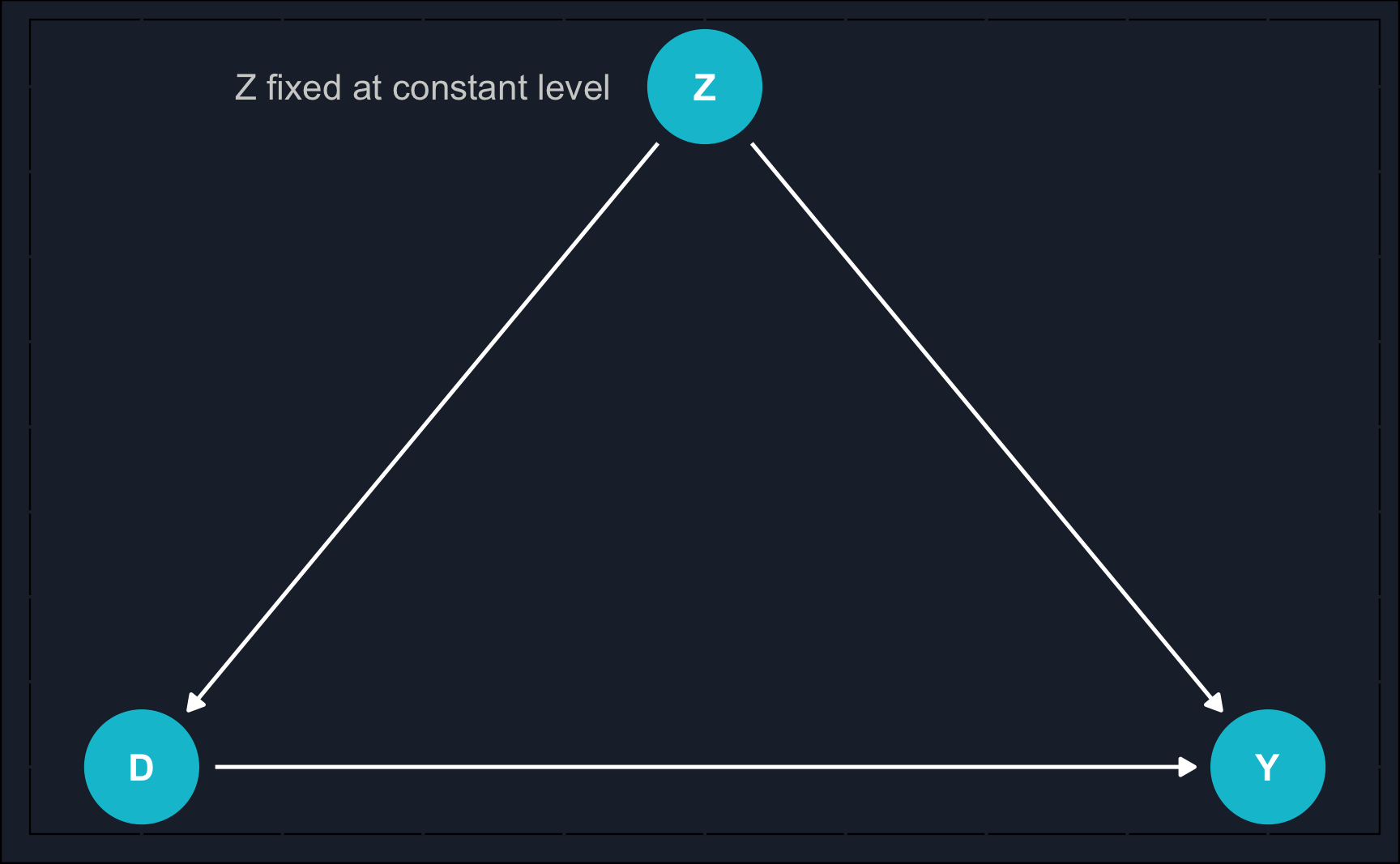
Effect of D on Y is confounded by variation in Z. In other words, there are two paths from D to Y, one direct path and a backdoor path via Z.

By now, you might recognize what kind of problem the DAG depicts: confounding. A variable $Z$ confounds the relationship between $X$ and $Y$ and to estimate the causal effect of $X$ on $Y$, we need to close the backdoor path of $X$ to $Y$ via $Z$.

Idea of Matching

One of the options to close the backdoor is matching, which covers any method attempting to equate or balance the distribution of covariates in treatment and control group. Simply put, the goal of matching is to compare apple to apples and after treatment make treatment and control group as similar as possible (of course, except for the treatment value).

In a way, matching is an alternative to using regression to close backdoors and neither is better or worse, in fact, they can even be combined. But for now, let us focus on matching and understand what it really it is, what kind of matching methods are popular and how they can be applied in R.

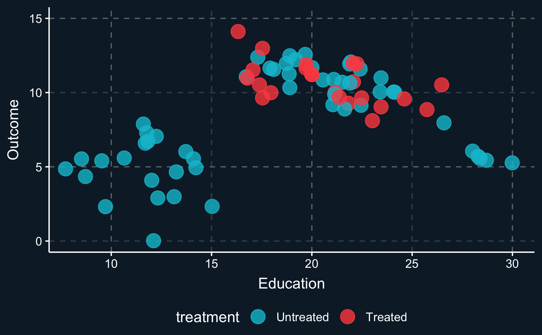
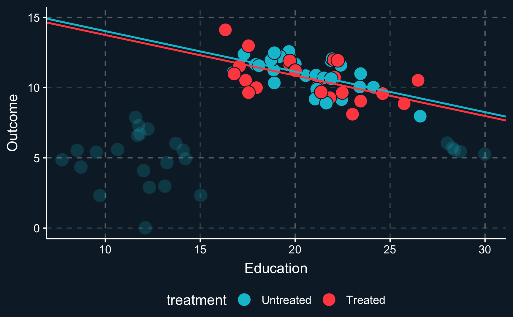
Let us assume you would like to study a phenomena and only have observational data that looks like this. $Z$ (education) is a covariate, $Y$ is the outcome and the color of the data points shows if a unit has been treated or not. From the first glance you can already see that the data does not look as if you would expect in a randomized experiment. For values of $Z$ in the middle range, there are both treated and untreated cases, but for values at the lower and upper range there are only untreated cases. That is an indication that $Z$ confounds the relationship between $D$ and $Y$.

Just imagine your measuring an arbitrary outcome and an arbitrary treatment confounded by years of education. When we plot the initial situation we see that for a low level of education and for a high level of education there are no treated observations. In causal inference lingo, treatment assignment is not independent from other factors, it is endogenous.

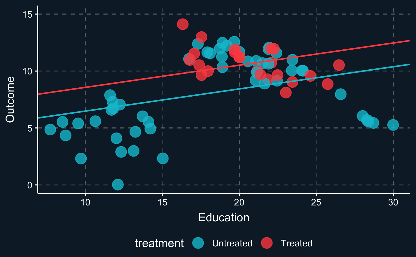
When we plot one line through all blue and one line through all red points and check the difference between the two lines, we see that there is substantial difference between both groups. This difference is what we would get as a treatment effect when we run a regression on all points. It indicates a positive treatment effect as the red line is above the blue line.

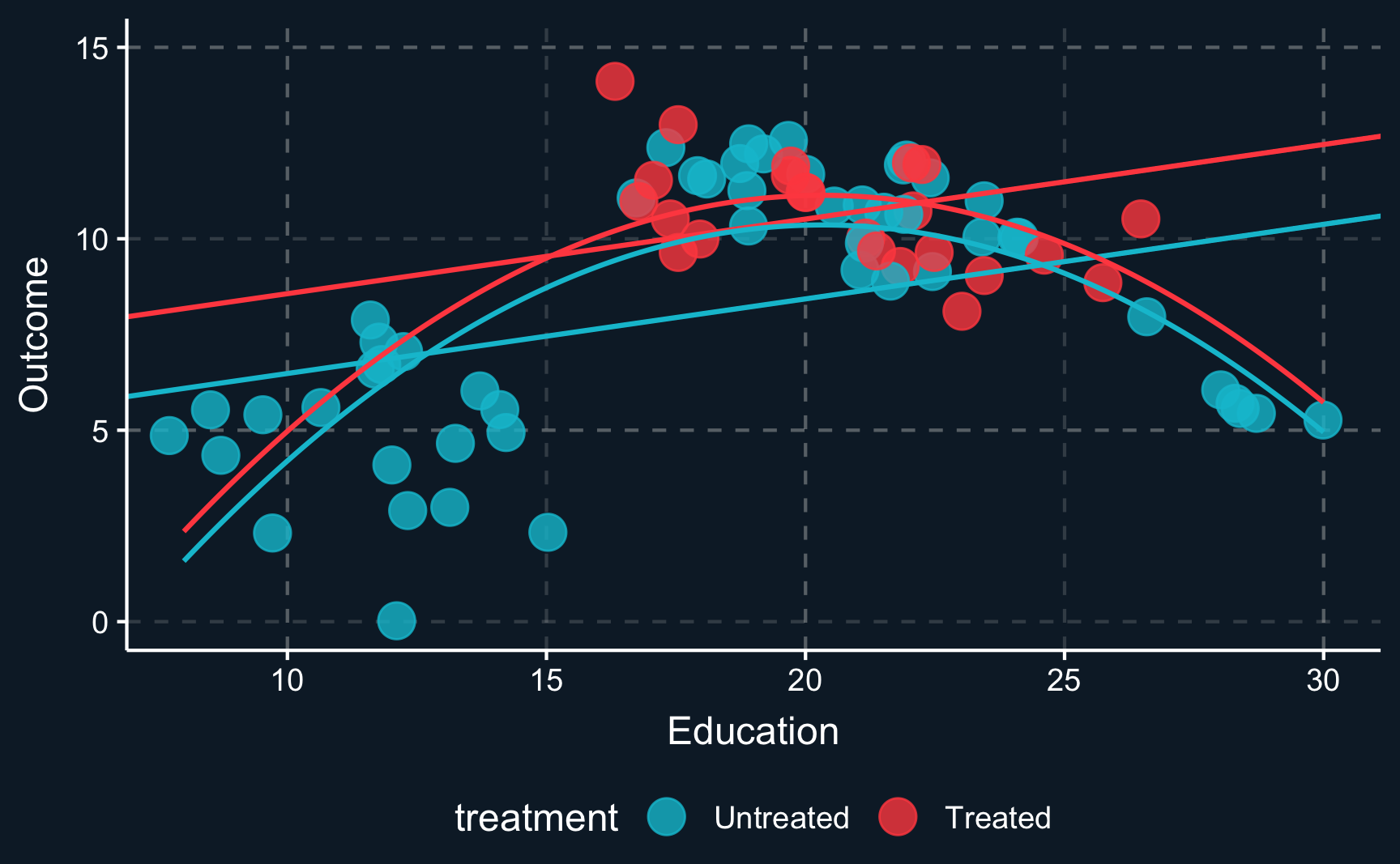
However, the lines clearly don’t fit the data very well because there does not seem to be a linear relationship. To account for non-linearities, you can introduce e.g. square terms to the regression, here $Z^2$ or $education^2$, respectively. Then, the fit improves, in particular for the untreated data points. But what happened to the treatment effect? There is still a positive treatment effect but now smaller in magnitude than the previous treatment effect. We already see that the estimate is highly dependent on the choice of our particular model. This is why we should always put a lot of consideration into choosing the right model (which is not necessarily the one with the largest or most desired treatment effect).

But we still have not really dealt with the fact that there are some regions where there are only units from one group. So let’s think about what we would have to do to adjust for the confounder $Z$. Ideally, we would like to compare treated and control group in an area where both groups are present. So the lower and upper region should actually be left out. Only where there is overlap of both groups, we can compare apples with apples. Focusing only on this (somewhat arbitrary) data points and drawing the lines and curves for both specifications of the regression, we get another different result. Now it seems, that there is a really small (probably ignorable) negative effect.

So, how do we know what units to select, especially when there is more than one dimension? We will explore some techniques in the following sections but the short answer is: we need to create a balance for values of all confounding variables treatment and control group, i.e. treatment and control group should be as similar as possible. And of course, we also need to assume, that all confounding variables are observed.

Subclassification Estimator

Although rarely used in practice, the subclassification estimator is an intuitive way of thinking about matching comparable observations and thereby controlling for confounders.

Essentially, the subclassification estimator estimates local treatment effects withing small groups that share the same values for (confounding) covariates. Sometimes, values does not need to be the same but only similar, e.g. for continuous variables like age it is very unlikely to find another observation unit with the exact same birthday, so you would define e.g. a birthyear. By only comparing observations in a small subgroup as defined by the covariates, conditional independence is ensured as there is no variation in the confounding variable.

Imagine, that a treatment was not randomly assigned for women and men and sex also plays a role for the outcome as well. One imaginary example could be the effect of a trainee program on later salary that was advertised more heavily to women and therefore more women participated. And being a women might also have an impact on salary. Then, we have the situation of a confounding variable, sex, and to control for it, we estimate a treatment effect for women and a treatment effect for men and average the effects weighted by the respective subsample size.

To check how that affects the estimated treatment effect we can simulate some data according to the following relationships.

# Number of observations
n <- 1e+3

# Variables
Z <- rbinom(n, 1, 0.5) # 0 => Male, 1 => Female
D <- rbinom(n, 1, p = if_else(as.logical(Z), 0.65, 0.35)) # 1 => Treat, 0 => Control
Y <- 0.2*D - 0.2*Z + rnorm(n, 5, 0.1) # => Salary

# Create tibble
df <- tibble(
  Z = Z,
  D = D,
  Y = Y
)

$D = participation$
$Z = sex$
$Y = salary$

As you can see both $D$ and $Y$ are related to $Z$ and $Y$ is influenced by both $D$ and $Z$. But we are only interested in isolating the effect of $D$ on $Y$. From the commands, we know that the true causal effect of $D$ on $Y$ is 0.2.

Let’s see what a naive comparison would return, where we would just compare average salary of the individuals who have participated in the trainee program are compared to the individuals who have not participated.

Accessing with base R

To access only certain elements of a table you can use table[row,col]. You can also use the $ operator to access columns.

# Naive comparison
E_0 <- mean(df[df$D==F, ]$Y) # control group
E_1 <- mean(df[df$D==T, ]$Y) # treatment group
E_1 - E_0

[1] 0.14

It is generally more convenient to use the lm() command.

# Regression of Y on D
summary(lm(Y ~ D, df))


Call:
lm(formula = Y ~ D, data = df)

Residuals:
    Min      1Q  Median      3Q     Max 
-0.3684 -0.0924  0.0006  0.0897  0.3576 

Coefficients:
            Estimate Std. Error t value Pr(>|t|)    
(Intercept)  4.92786    0.00597   825.9   <2e-16 ***
D            0.14334    0.00826    17.4   <2e-16 ***
---
Signif. codes:  0 '***' 0.001 '**' 0.01 '*' 0.05 '.' 0.1 ' ' 1

Residual standard error: 0.13 on 998 degrees of freedom
Multiple R-squared:  0.232, Adjusted R-squared:  0.231 
F-statistic:  301 on 1 and 998 DF,  p-value: <2e-16

Due to confounding, the naive comparison cannot reconstruct our implemented treatment effect (= 0.2, defined when we simulated the outcome variable) and is off. We should get closer if we account for confounding by taking averages treatment effects for men and women separately.

# Subclassification estimator (subclasses: Z = 0 and Z = 1)
# E(Z, D)
E_00 <- mean(df[(df$Z==F & df$D==F), ]$Y) # control men
E_10 <- mean(df[(df$Z==T & df$D==F), ]$Y) # control women
E_01 <- mean(df[(df$Z==F & df$D==T), ]$Y) # treatment men
E_11 <- mean(df[(df$Z==T & df$D==T), ]$Y) # treatment women

# Weighted by K (proportion of female/male)
K <- mean(Z)

K*(E_11-E_10) + (1-K)*(E_01 - E_00)

[1] 0.2

And in fact, now we are really close to the true treatment effect. The remaining difference is caused by randomness in our sampling process.

This way, we have closed the backdoor and are able to retrieve the causal effect. However, note that the effect can only be causally interpreted, if sex is the only confounding variable. If there are more confounders, we have to build smaller groups that are defined by value combinations of all confounders, which will at some point lead groups that are extremely small or maybe even empty. This is called the curse of dimensionality and we’ll deal with it in the following sections.

Matching as a Concept

In the previous section, observations from treatment and control group were required to have equal covariates. But matching can also take other forms that are less strict. Generally, we are trying to select observations in the control group that are similar to those in the treated group. To do so, we need to define what similar means. By enforcing treatment and control group to have little variation in the matching variables, we close the backdoors. When the backdoor variable does not vary or varies only very little, it cannot induce changes in treatment and outcome. So, when we suppress this variation in the backdoor variable, we can interpret the effect from treatment to outcome as causal.

There are many ways and methods to conduct this and we will go through some of them. But let’s first define matching conceptually.

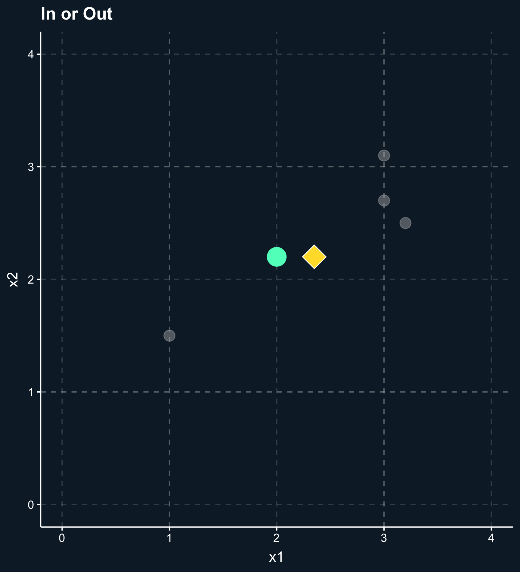
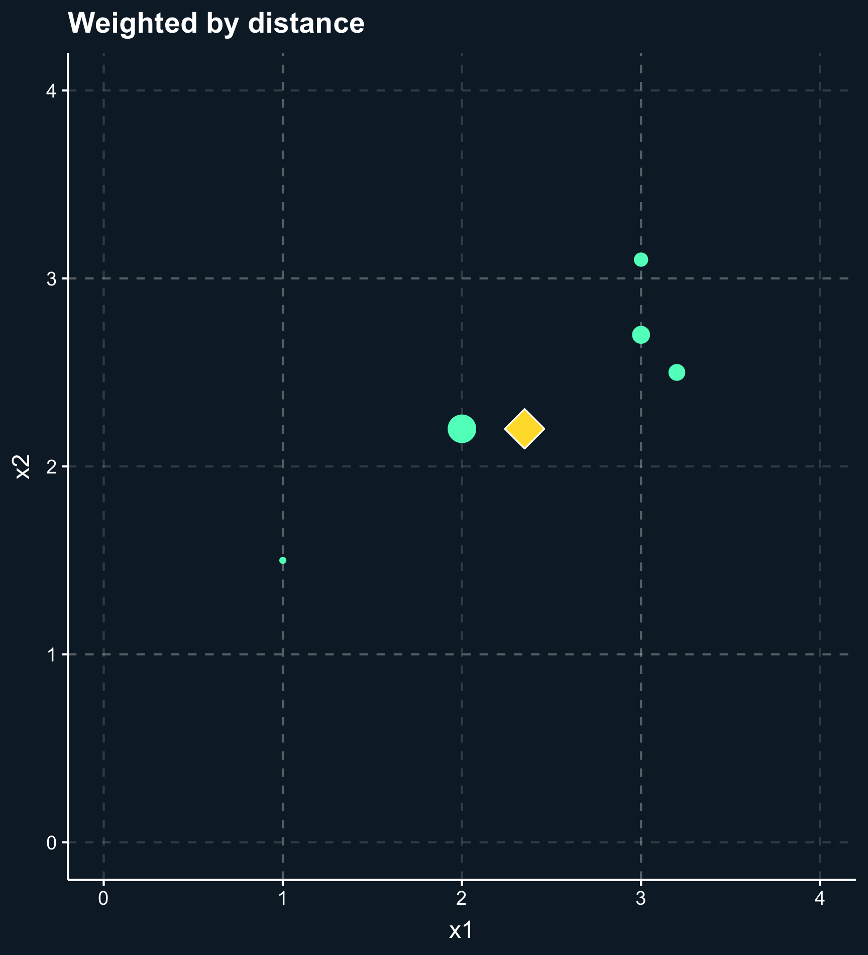
In general, the outcome of a matching method are weights for each observation based on one or several matching variables. For some matching methods the weights are either 0 or 1 (in or out), but there are also a lot of methods that give weights between 0 and 1 (less and more important) to observations.

The matching variables need to cover the variables that can - when adjusted on - block all backdoor paths between our treatment variable and the outcome. Then, the treatment effect is computed as a weighted mean of the outcomes for the treatment and control group.

Matching methods can be classified into two main approaches: matching based on (1) distance and matching based on (2) propensity scores.

Distance: observations are similar if they have similar covariates (or more specific: similar values for the matching variables). This approach minimizes the distance between observations in treatment and control group based on their covariate values.
Propensity: observations are similar if they are equally likely to be treated, i.e. matching variables are used to build a prediction model of how likely an observation is to be in treatment group, regardless whether it actually is in the treatment or control group.

As you can also see in the plot, another difference across methods is whether observations are compared to matches, which classify other observations as either in our out or compared to matched weighted samples, where each observation obtains a different weight depending on how close they are. For matches, you have to decide how many to include or what the worst acceptable match is while for matched weighted samples you need to decide how weights decay with distance.

Initial situation: one treated observation and five potential matches from the control group.

The closest match is selected to compute treatment effect. Match is indicated by color of data point.

Several units are selected and weighted by their distance. Weight is indicated by size of data point.

We can now outline a structure for the general process of matching that applies to all methods.

First, it starts with some kind of preprocessing, which is a “manual” part, where you use all information about the causal mechanisms that you have. Essentially, it forces you to look at the DAG you can draw based on all your theoretical knowledge and thoughts, and particularly what you know about the treatment assignment. In randomized studies, you do not have to take any preprocessing steps.
Then, using this preprocessed data you can build your model to estimate the treatment effect.

Now, let’s look at some methods in detail and afterwards get more application-oriented.

Single Matching Variable

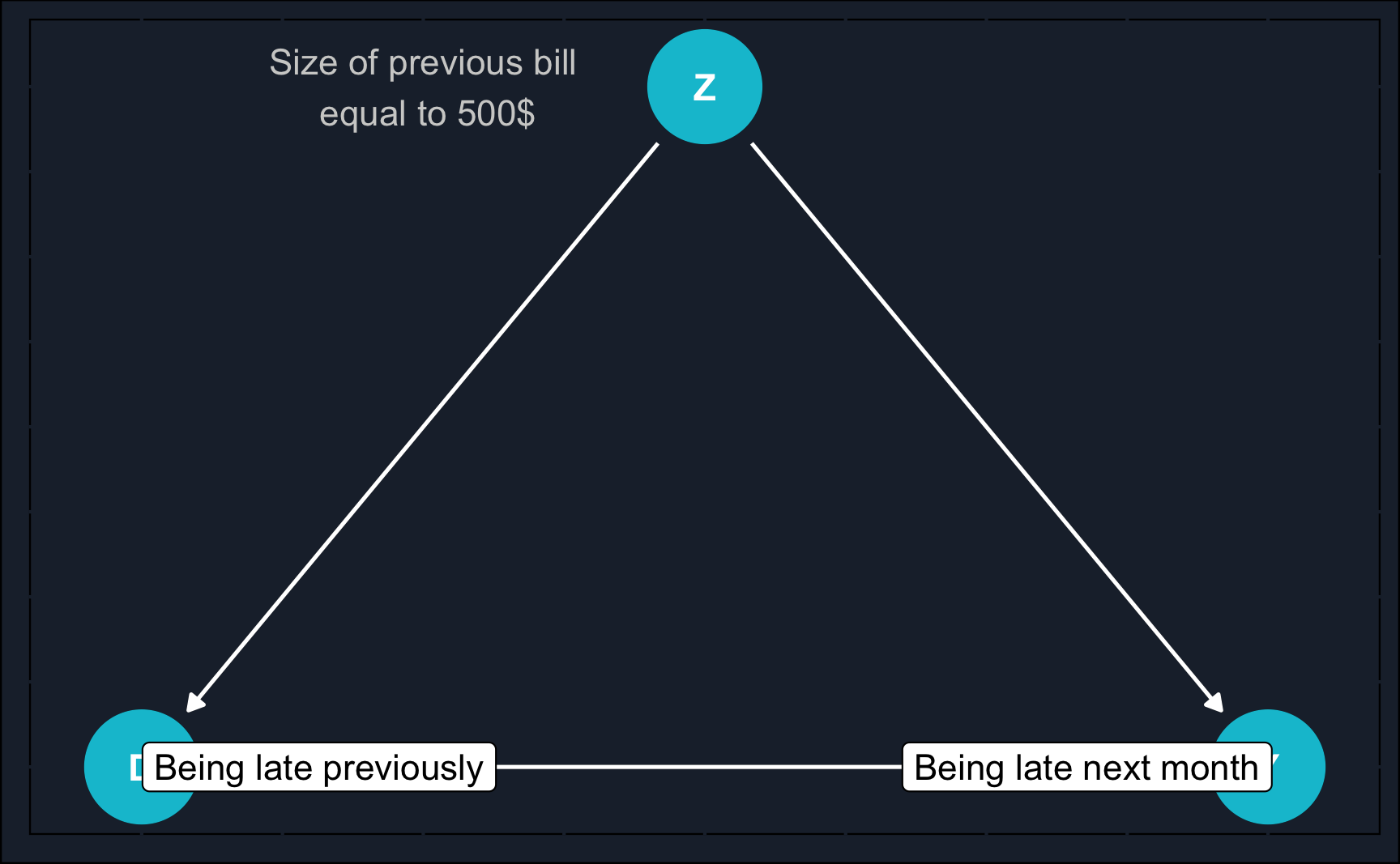
The most simple scenario would be to match on a single variable. In practice, it is rare that only one variable is a potential confounder but for the purpose of practice, we’ll start with this scenario. Consider a scenario where you are employed by a bank and need to make a decision regarding whether to issue a credit card to a customer who has previously experienced credit difficulties.

Let’s delve into specific methods in depth, and then transition towards a more practical application-focused approach.

Generic DAG with matching. By fixing the level of confounder, backdoor is closed and valid estimation of causal treatment effect for that specific group at level of confounder.

Applied to credit card example. Effect of being late on settling credict card debt in the past on being late again. Confounded by size of credit card debt. It could be suspected that customers with higher debts in the past are unlikely to be financially recovered by now. Therefore, we have to condition on the level of the previous bill.

(Coarsened) Exact Matching

When you think of the previous credit card example, you might have asked yourself:

How likely is it that when fixing a continuous variable such as previous bill, we can find matching treatment and control observations? I.e. we have a treated and an untreated observation with exactly the same previous bill.

It is in fact very unlikely, and to address this issue we rely on coarsening continuous variables. That means, we create different levels/bins for the size of the previous bill, which could be for example: 1-50€, 51-250€, 251-1000€ and so on. This increases the likelihood of finding matches substantially. However, we also lose a bit of precision. In general: the wider the bins, the more matches but the less precision.

Now, however, there might be even more than one match for a particular observation. In this case, you could compute an average or weight the matches based on their distance to the focal observation.

Nearest-Neighbor Matching

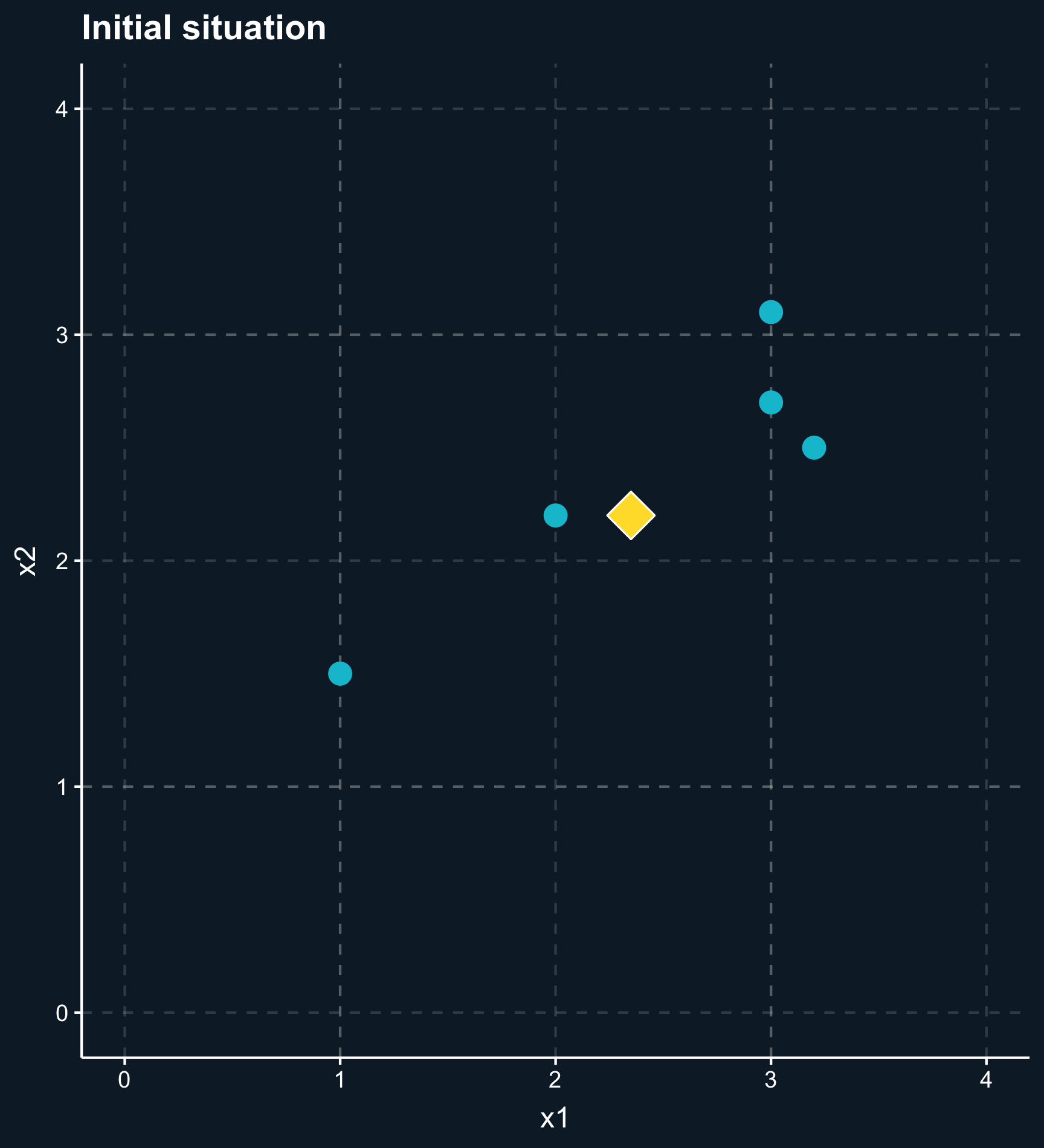
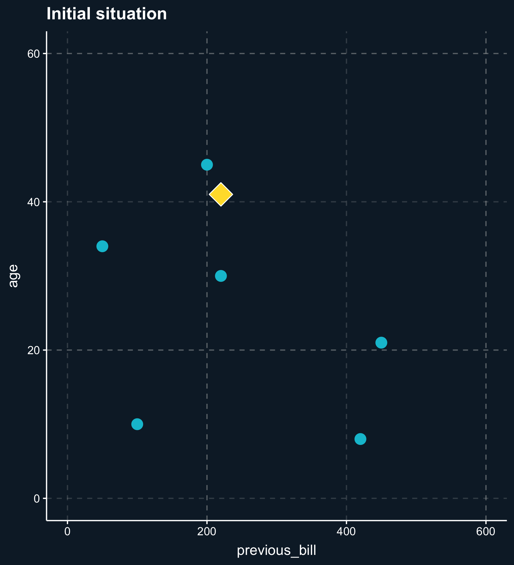
Distance also plays a crucial role when taking more than one matching variable into account. Let’s add the variable $age$ and plot the two dimensions.

Less less strict than exact or coarsened matching, matching on distance finds observations that are close. The distance between observations is computed using distance measures such as the distance or the Euclidean distance and close matches are identified e.g. by nearest-neighbor matching or by using kernel weights.

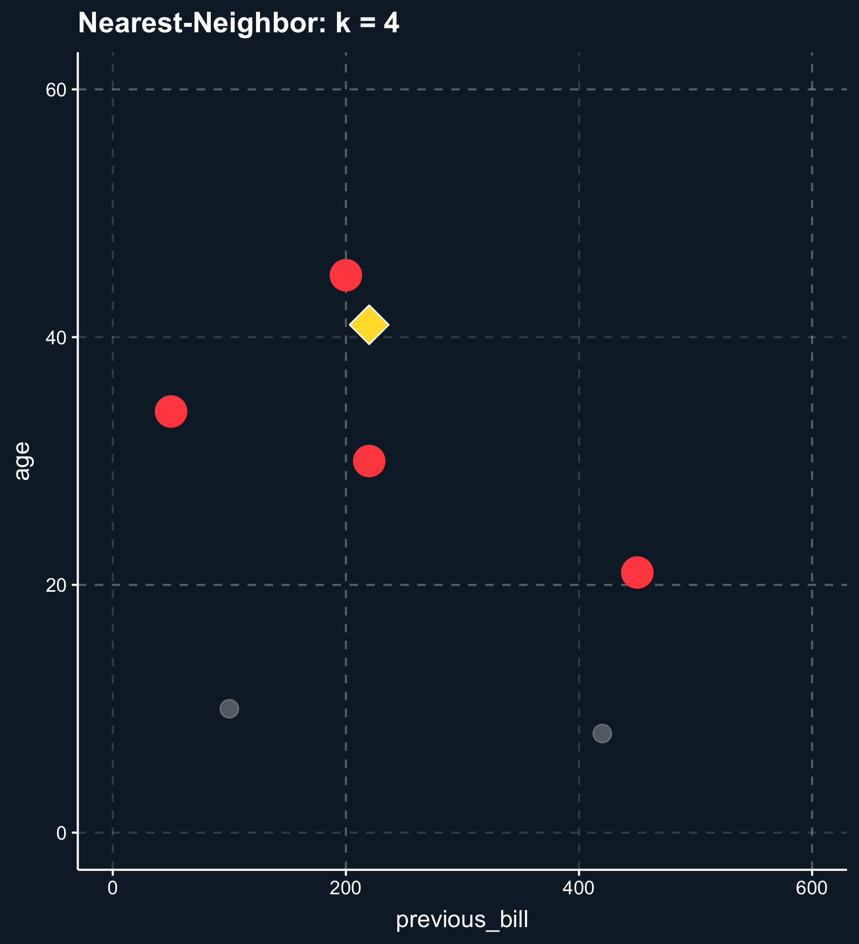
Initial situation: six potential matches.

Matches are only accepted if they fall into specified vicinity.

Using nearest-neighbor matching, for each two observations, a scalar is returned calculated from the distances of all matching variables. Based on that value, $k$ matching observations are selected to build the control group. If $k \neq 1$, you also have to decide whether to weight the control observations on their distance. Weighting the observations makes the approach less sensitive to the choice of $k$ because less importance observations are down-weighted. Eventually the weights goes to zero.

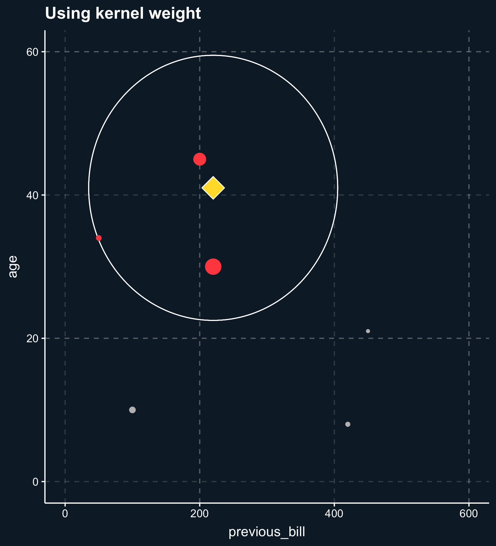
Kernel weights are similar but define a vicinity observations have to fall into.

Propensity score

With an increasing number of matching variables nearest-neighbors matching becomes unfeasible, as well. To reduce the dimensionality onto one dimension, for each observation a propensity score can be computed. The propensity score expresses the estimated probability of treatment. In absence of selection bias, propensity scores should be very similar across treatment and control group. Thinking back to our probability chapter, the propensity score is:

\[ P(D_i = 1|\mathbf{X}_i) \]

We’ll discuss how to use it later in detail but essentially, we exploit that there are units in the treatment group that were unlikely to be treated and vice versa. The most recommended method that uses propensity scores as matching input is called inverse probability weighting and weights each observation by the inverse of the probability for its own treatment status. Simply put, atypical observations receive a high weight, so if you were actually treated which was unlikely based on your covariates, you receive a high weight.

Application

Multiple Matching Variables

Let us imagine, you want to reduce the number of sick days in your company by implementing a health program that employees are free to participate in. By learning about how to improve their health, you expect your employees to call in sick less frequently.

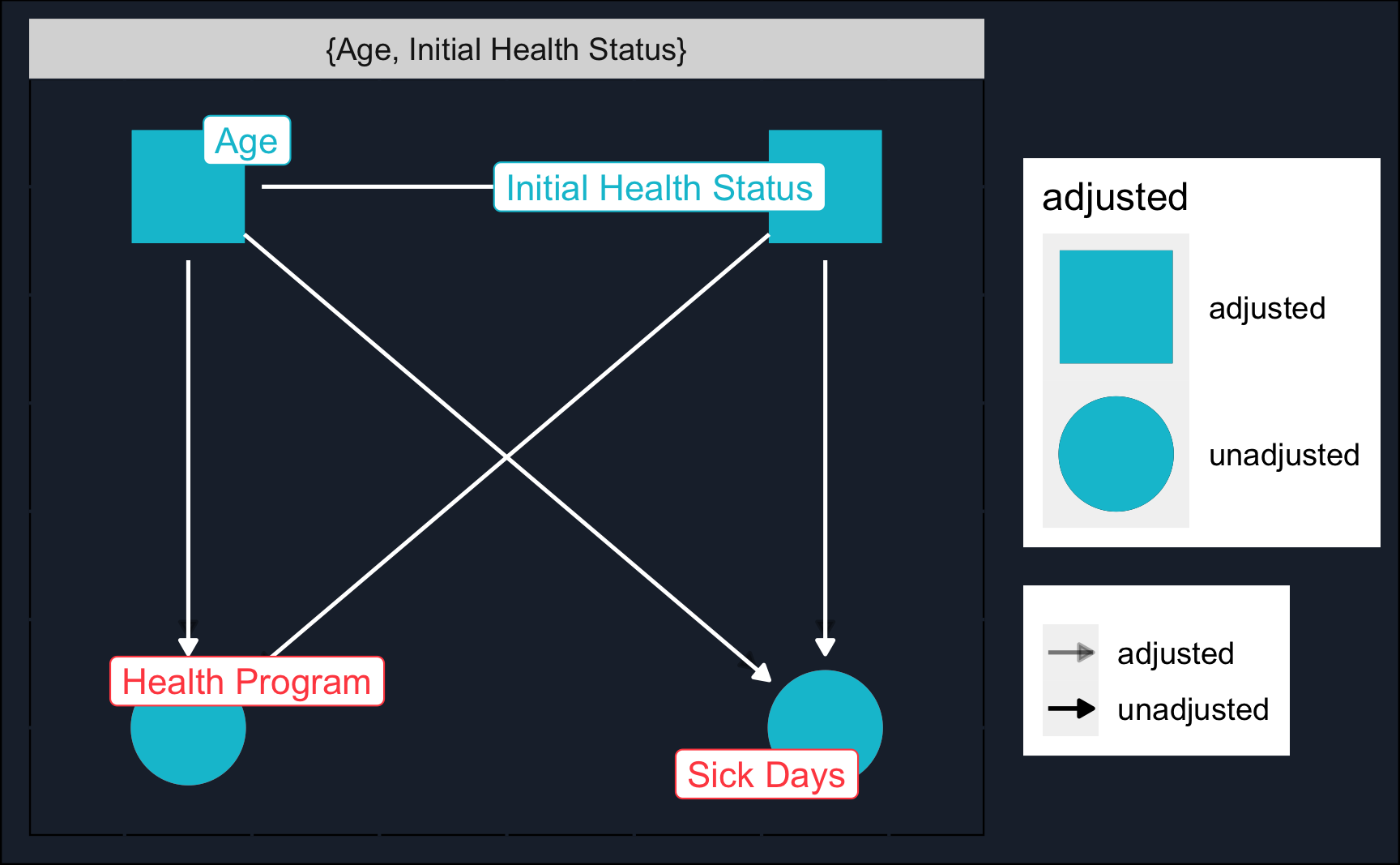
Now you already see that the treatment, participation in the health program, is on a voluntary basis and therefore treatment assignment might be confounded by variables such as age and initial health status. Older and sicker people might be more interested to learn about techniques and procedures to improve their health and also might benefit more from the program. Also, initial health status might be affected by age. Let’s assume for demonstration purposes that these are the only confounding factors. In practice, there might be more, however.

We can use a DAG to think about the correct identification strategy. Using dagitty and ggdag we see that we need to close two backdoor paths: initial health status and age.

# Load packages
library(dagitty)
library(ggdag)

# Define DAG
dag_model <- 'dag {
  bb="0,0,1,1"
  "Health Program" [exposure,pos="0.25,0.2"]
  "Initial Health Status" [pos="0.35,0.25"]
  "Sick Days" [outcome,pos="0.35,0.2"]
  Age [pos="0.25,0.25"]
  "Initial Health Status" -> "Health Program"
  "Initial Health Status" -> "Sick Days"
  Age -> "Health Program"
  Age -> "Initial Health Status"
  Age -> "Sick Days"
}'

# DAG with adjustment sets (and custom layout)
ggdag_adjustment_set(dag_model, shadow = T, text = F) +
  guides(color = "none") +  # Turn off legend
  theme_dag_cds() + # custom layout (can be left out)
  geom_dag_point(color = ggthemr::swatch()[2]) + # custom color, can take any color
  geom_dag_text(color = NA) +
  geom_dag_edges(edge_color = "white") +
  geom_dag_label_repel(aes(label = name))

DAG showing what needs to be accounted for.

Let’s load the data (you probably have to change the path) and have a glance at it.

# Read data
df <- readRDS("../../datasets/health_program.rds")

# Show data 
df

True Treatment Effect

Because the data is simulated, we know the true treatment effect: 0.5

Compare it to the estimates in the following sections!

A naive estimate would be obtained by just regressing sick_days on health_program.

# Naive estimation (not accounting for backdoors)
model_naive <- lm(sick_days ~ health_program, data = df)
summary(model_naive)


Call:
lm(formula = sick_days ~ health_program, data = df)

Residuals:
   Min     1Q Median     3Q    Max 
-7.546 -1.546 -0.248  0.752 20.454 

Coefficients:
                   Estimate Std. Error t value Pr(>|t|)    
(Intercept)          7.2483     0.0328   220.9   <2e-16 ***
health_programTRUE   1.2980     0.0464    27.9   <2e-16 ***
---
Signif. codes:  0 '***' 0.001 '**' 0.01 '*' 0.05 '.' 0.1 ' ' 1

Residual standard error: 2.3 on 9998 degrees of freedom
Multiple R-squared:  0.0725,    Adjusted R-squared:  0.0724 
F-statistic:  781 on 1 and 9998 DF,  p-value: <2e-16

The naive estimate is far off. But we already suspected that treatment assignment was not random, so let’s see if we can improve the validity of our estimation using matching procedures.

(Coarsened) Exact Matching

Again, in case of exact matching, only observations that share the same values in (coarsened) matching variables are matched in. To perform Coarsened Exact Matching (CEM) you can use the MatchIt package in R. We provide a formula containing our treatment dependent on the matching variables, the data, what method to use ('cem' = Coarsened Exact Matching) and what estimate we are interested in. Please note we regress the treatment on the matching variables. The outcome variable is not included at this stage.

# Load 'MatchIt' library
library(MatchIt)

# Without specifying coarsening
# (1) Matching
cem <- matchit(health_program ~ age + sick_days_before,
               data = df, 
               method = 'cem', 
               estimand = 'ATE')

Using the summary() function we can check how well balanced the covariates are compared to before. The balance before is titled Summary of Balance for All Data and after Summary of Balance for Matched Data. In this case, they are almost perfectly balanced after matching.

# Covariate balance
summary(cem)


Call:
matchit(formula = health_program ~ age + sick_days_before, data = df, 
    method = "cem", estimand = "ATE")

Summary of Balance for All Data:
                 Means Treated Means Control Std. Mean Diff. Var. Ratio eCDF Mean eCDF Max
age                       46.3          44.7            0.17       0.94     0.045    0.067
sick_days_before           4.2           3.5            0.37       1.54     0.034    0.177

Summary of Balance for Matched Data:
                 Means Treated Means Control Std. Mean Diff. Var. Ratio eCDF Mean eCDF Max Std. Pair Dist.
age                       45.5          45.5          -0.001          1     0.002    0.009            0.11
sick_days_before           3.8           3.8           0.008          1     0.001    0.017            0.10

Sample Sizes:
              Control Treated
All              5006    4994
Matched (ESS)    4707    4700
Matched          5002    4941
Unmatched           4      53
Discarded           0       0

Now, we can use the matched data and see how the coefficient changes. Actually, it changes quite a lot. Even when at first glance, the covariates were not too different before matching.

# Use matched data
df_cem <- match.data(cem)

# (2) Estimation
model_cem <- lm(sick_days ~ health_program, data = df_cem, weights = weights)
summary(model_cem)


Call:
lm(formula = sick_days ~ health_program, data = df_cem, weights = weights)

Weighted Residuals:
   Min     1Q Median     3Q    Max 
-8.319 -1.447 -0.483  0.960 14.772 

Coefficients:
                   Estimate Std. Error t value Pr(>|t|)    
(Intercept)          7.5864     0.0318   238.9   <2e-16 ***
health_programTRUE   0.5296     0.0450    11.8   <2e-16 ***
---
Signif. codes:  0 '***' 0.001 '**' 0.01 '*' 0.05 '.' 0.1 ' ' 1

Residual standard error: 2.2 on 9941 degrees of freedom
Multiple R-squared:  0.0137,    Adjusted R-squared:  0.0136 
F-statistic:  138 on 1 and 9941 DF,  p-value: <2e-16

Looking at our matching command matchit() you might have noticed that we did not specify any cut points to perform the coarsened matching. Instead the MatchIt module took care of that in the background. But we can also choose to specify cut points.

We’ll see that we are able to decrease the imbalance, but not to the same degree as the algorithm did it. Feel free to check out if you can get any closer.

# Custom coarsening
# (1) Matching
cutpoints <- list(age = seq(25, 65, 15), sick_days_before = seq(3, 22, 5))
cem_coars <- matchit(health_program ~ age + sick_days_before,
                     data = df, 
                     method = 'cem', 
                     estimand = 'ATE',
                     cutpoints = cutpoints)

# Covariate balance
summary(cem_coars)


Call:
matchit(formula = health_program ~ age + sick_days_before, data = df, 
    method = "cem", estimand = "ATE", cutpoints = cutpoints)

Summary of Balance for All Data:
                 Means Treated Means Control Std. Mean Diff. Var. Ratio eCDF Mean eCDF Max
age                       46.3          44.7            0.17       0.94     0.045    0.067
sick_days_before           4.2           3.5            0.37       1.54     0.034    0.177

Summary of Balance for Matched Data:
                 Means Treated Means Control Std. Mean Diff. Var. Ratio eCDF Mean eCDF Max Std. Pair Dist.
age                       45.6          45.3           0.025       0.99     0.006    0.016            0.47
sick_days_before           3.9           3.7           0.118       1.09     0.012    0.090            0.59

Sample Sizes:
              Control Treated
All              5006    4994
Matched (ESS)    4857    4840
Matched          5006    4989
Unmatched           0       5
Discarded           0       0

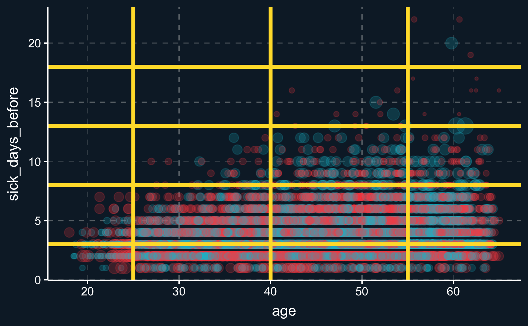
We can also visualize the subsamples and see how data points are weighted. Weights depend on how many treated and control units there are in a specific subsample. You can see that in the top-right corner, for example. From the plot we can also see that the cut-points specified by us are too broad as matches could be way closer.

# Use matched data
df_cem_coars <- match.data(cem_coars)

# Plot grid
ggplot(df_cem_coars, aes(x = age, y = sick_days_before,
                         size = weights, color = as.factor(health_program))) +
  geom_point(alpha = .2) +
  geom_abline(data.frame(y = cutpoints$sick_days_before),
              mapping = aes(intercept = y, slope = 0), 
              linewidth = 1.5, color = ggthemr::swatch()[5]) +
  geom_vline(data.frame(y = cutpoints$age),
              mapping = aes(xintercept = y),
             linewidth = 1.5, color = ggthemr::swatch()[5]) +
  theme(legend.position = "none")

Coarsening: each subsample only contains similar units. If there are just a few treated observations, the toal weight of control units is lower for a specific subsample.

With custom coarsening, we again get another coefficient. It could indicate that this way, backdoors are not properly closed because we our cut points were defined too broadly.

# (2) Estimation
model_cem_coars <- lm(sick_days ~ health_program, data = df_cem_coars, 
                      weights = weights)
summary(model_cem_coars)


Call:
lm(formula = sick_days ~ health_program, data = df_cem_coars, 
    weights = weights)

Weighted Residuals:
   Min     1Q Median     3Q    Max 
-8.401 -1.445 -0.307  0.839 26.167 

Coefficients:
                   Estimate Std. Error t value Pr(>|t|)    
(Intercept)          7.5126     0.0330   227.6   <2e-16 ***
health_programTRUE   0.7530     0.0467    16.1   <2e-16 ***
---
Signif. codes:  0 '***' 0.001 '**' 0.01 '*' 0.05 '.' 0.1 ' ' 1

Residual standard error: 2.3 on 9993 degrees of freedom
Multiple R-squared:  0.0253,    Adjusted R-squared:  0.0252 
F-statistic:  260 on 1 and 9993 DF,  p-value: <2e-16

Nearest-Neighbor matching

For nearest neighbor matching, the difference between two observations based on multiple variables is computed and reduced to a scalar. One of the most popular distance measures used to find so called nearest neighbors is the Mahalanobis distance.

Again, we use MatchIt to conduct the matching process. We just have to change a few arguments and decide to use the Mahalanobis distance. Then, we check how similar treatment and control group are after matching. The result differs from (coarsened) exact matching but again, we have almost perfect balance.

# (1) Matching
# replace: one-to-one or one-to-many matching
nn <- matchit(health_program ~ age + sick_days_before,
              data = df,
              method = "nearest", # changed
              distance = "mahalanobis", # changed
              replace = T)

# Covariate Balance
summary(nn)


Call:
matchit(formula = health_program ~ age + sick_days_before, data = df, 
    method = "nearest", distance = "mahalanobis", replace = T)

Summary of Balance for All Data:
                 Means Treated Means Control Std. Mean Diff. Var. Ratio eCDF Mean eCDF Max
age                       46.3          44.7            0.17       0.94     0.045    0.067
sick_days_before           4.2           3.5            0.33       1.54     0.034    0.177

Summary of Balance for Matched Data:
                 Means Treated Means Control Std. Mean Diff. Var. Ratio eCDF Mean eCDF Max Std. Pair Dist.
age                       46.3          46.3          -0.000          1     0.001    0.005           0.011
sick_days_before           4.2           4.2           0.001          1     0.000    0.002           0.002

Sample Sizes:
              Control Treated
All              5006    4994
Matched (ESS)    1769    4994
Matched          2643    4994
Unmatched        2363       0
Discarded           0       0

And also the estimated average treatment effect is very similar to the one obtained by (default) CEM.

# Use matched data
df_nn <- match.data(nn)

# (2) Estimation
model_nn <- lm(sick_days ~ health_program, data = df_nn, weights = weights)
summary(model_nn)


Call:
lm(formula = sick_days ~ health_program, data = df_nn, weights = weights)

Weighted Residuals:
   Min     1Q Median     3Q    Max 
-8.942 -1.546 -0.546  1.237 29.865 

Coefficients:
                   Estimate Std. Error t value Pr(>|t|)    
(Intercept)          8.0182     0.0486  164.84   <2e-16 ***
health_programTRUE   0.5280     0.0602    8.78   <2e-16 ***
---
Signif. codes:  0 '***' 0.001 '**' 0.01 '*' 0.05 '.' 0.1 ' ' 1

Residual standard error: 2.5 on 7635 degrees of freedom
Multiple R-squared:  0.00999,   Adjusted R-squared:  0.00986 
F-statistic: 77.1 on 1 and 7635 DF,  p-value: <2e-16

Curse of dimensionality

With exact matching and nearest-neighbor matching you quickly run into the curse of dimensionality as your number of covariates grows. If you want to find matches based on very few dimensions, you are way more likely to find them as opposed to matches on a high number of dimensions, where it is very likely that you actually don’t find any matches at all.

Regarding exact matching, consider for example the situation with two covariates with each five distinct values. Then any observations will fall into one of 25 different cells that are given by the covariate value grid. And now imagine ten covariates with three different values: it already creates ~60k cells, which increases the likelihood of a cell being populated by only one or zero observations substantially. Then, estimation of treatment effects is not possible for many of the observations.

Inverse Probability weighting

One way to deal with the curse of dimensionality is to use inverse probability weighting (IPW). We already mentioned it above, but let’s go into more detail.

Estimating Propensity Score

We start by understanding what probability in inverse probability means. It is the predicted probability of treatment assignment based on the matching variables. So staying in the health program example, we use age and initial health status to predict how likely an employee is to participate in the health program. What we expect is that older and initially more sick people are more likely to participate opposed to younger and healthy people. To model this relationship, we could use for example logistic regression, a regression that predicts an outcome between zero and one. But you are also free to use any classification model that is out there, as here we are not only interested in explaining effects but only in obtaining the probability of treatment, also known as propensity score.

Here, we will use a logistic regression for prediction. A logistic regression, opposed to a linear regression, is designed for outcomes that are between 0 and 1, such as probabilities. The coefficients are a bit more difficult to interpret, so we’ll leave that for now. But what we see is, that age and sick_days_before are relevant and positive predictors for the probability of treatment.

# (1) Propensity scores
model_prop <- glm(health_program ~ age + sick_days_before,
                  data = df,
                  family = binomial(link = "logit"))
summary(model_prop)


Call:
glm(formula = health_program ~ age + sick_days_before, family = binomial(link = "logit"), 
    data = df)

Coefficients:
                 Estimate Std. Error z value Pr(>|z|)    
(Intercept)       -1.1851     0.1000  -11.85  < 2e-16 ***
age                0.0102     0.0021    4.87  1.1e-06 ***
sick_days_before   0.1898     0.0116   16.37  < 2e-16 ***
---
Signif. codes:  0 '***' 0.001 '**' 0.01 '*' 0.05 '.' 0.1 ' ' 1

(Dispersion parameter for binomial family taken to be 1)

    Null deviance: 13863  on 9999  degrees of freedom
Residual deviance: 13497  on 9997  degrees of freedom
AIC: 13503

Number of Fisher Scoring iterations: 4

For each observation we can compute a probability and add it to a table. It is important to specify type = "response" in the predict() command to obtain probabilities.

# Add propensities to table
df_aug <- df %>% mutate(propensity = predict(model_prop, type = "response"))

Having obtained the propensity score, you could again measure distances like described above and select matches. In fact, that is widely used matching method, known as propensity score matching. However, there are several reasons why this is not a good identification strategy¹, mainly, because same propensity score does not imply that observations have the same covariate values and this could actually increase the imbalance. Note, however, that vice versa, covariate values indeed imply the same propensity score.

Weighting by Propensity Score

Instead inverse probability weighting (IPW) has proven to be a more precise method, particularly when the sample is large enough. So what do we do with the probability/propensity scores in IPW? We use the propensity score of an observation unit to increase or decrease its weights and thereby make some observations more important than others. The weight obtains as

\[ w_i = \frac{D_i}{\pi_i} + \frac{(1-D_i)}{(1-\pi_i)} \]

where only one of the terms is always active as $D_i$ is either one or zero. Now we should better understand what “inverse probability weighting” actually means. It weights each observation by its inverse of its treatment probability. Let’s compute it for our data.

# Extend data by IPW scores
df_ipw <- df_aug %>% mutate(
  ipw = (health_program/propensity) + ((1-health_program) / (1-propensity)))

# Look at data with IPW scores
df_ipw %>% 
  select(health_program, age, sick_days_before, propensity, ipw)

Imagine a case of an old employee with a very bad initial health status who chose to participate in the health program, i.e. $D_i=1$. Based on his/her covariates, it was very likely that he choose to participate and consequently, his propensity score will be rather high, let’s assume it was 0.8, for demonstration. Then his/her weight would equal $w_i = \frac{1}{0.8} = 1.25$.

Compared to that, what weight would a young and healthy person that choose to participate in the program obtain? Let’s say his/her probability of participating would be 0.2. Then, his/her weight would be $w_i = \frac{1}{0.2} = 5$. So we see, he/she would obtain a significantly higher weight.

In general, IPW weights atypical observations, like a young and healthy person deciding to participate, higher than typical observations. The same applies for both treatment and control group.

Running a linear regression with weights as provided by IPW yields a coefficient not as precise as the ones obtained by previous matching procedures.

# (2) Estimation
model_ipw <- lm(sick_days ~ health_program,
                data = df_ipw, 
                weights = ipw)
summary(model_ipw)


Call:
lm(formula = sick_days ~ health_program, data = df_ipw, weights = ipw)

Weighted Residuals:
   Min     1Q Median     3Q    Max 
-12.11  -2.31  -0.28   1.26  93.19 

Coefficients:
                   Estimate Std. Error t value Pr(>|t|)    
(Intercept)          7.7567     0.0352  220.12   <2e-16 ***
health_programTRUE   0.4213     0.0500    8.43   <2e-16 ***
---
Signif. codes:  0 '***' 0.001 '**' 0.01 '*' 0.05 '.' 0.1 ' ' 1

Residual standard error: 3.5 on 9998 degrees of freedom
Multiple R-squared:  0.00706,   Adjusted R-squared:  0.00697 
F-statistic: 71.1 on 1 and 9998 DF,  p-value: <2e-16

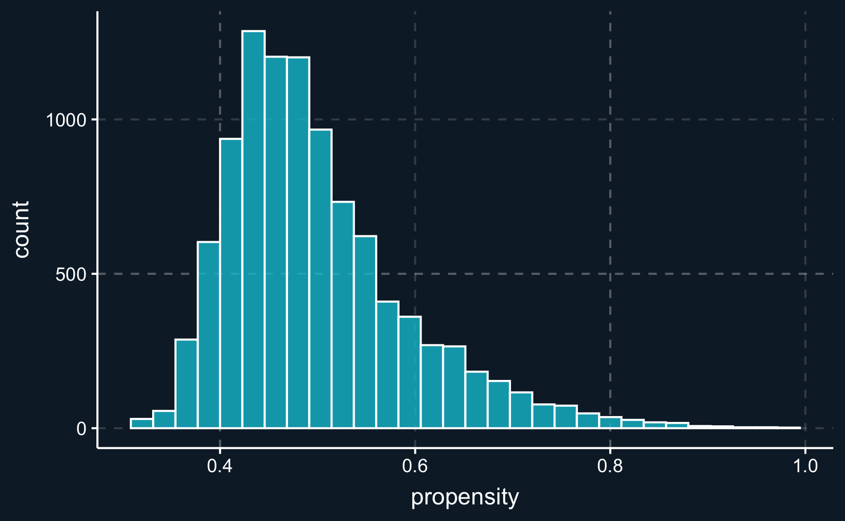
A reason for that could be that there are some extreme and very atypical observations with either very high or low probabilities. Those observations than get a very high weight.

# Plot histogram of estimated propensities
ggplot(df_aug, aes(x = propensity)) +
  geom_histogram(alpha = .8, color = "white")

Most predicted treatment probabilities are between 0.4 and 0.6. Only a few outliers.

# Looking for observations with highest weights
df_ipw %>% 
  select(health_program, age, sick_days_before, propensity, ipw) %>% 
  arrange(desc(ipw))

To avoid assigning extreme weights, a proposed best practice is to trim the sample² and filter out all observations with a propensity score less than 0.15 and higher than 0.85. Doing that,the coefficient is very close to the true treatment effect.

# Run with high weights excluded
model_ipw_trim <- lm(sick_days ~ health_program,
                data = df_ipw %>% filter(propensity %>% between(0.15, 0.85)),
                weights = ipw)
summary(model_ipw_trim)


Call:
lm(formula = sick_days ~ health_program, data = df_ipw %>% filter(propensity %>% 
    between(0.15, 0.85)), weights = ipw)

Weighted Residuals:
    Min      1Q  Median      3Q     Max 
-12.034  -2.180  -0.517   1.287  23.904 

Coefficients:
                   Estimate Std. Error t value Pr(>|t|)    
(Intercept)          7.6553     0.0324   236.1   <2e-16 ***
health_programTRUE   0.4776     0.0459    10.4   <2e-16 ***
---
Signif. codes:  0 '***' 0.001 '**' 0.01 '*' 0.05 '.' 0.1 ' ' 1

Residual standard error: 3.2 on 9956 degrees of freedom
Multiple R-squared:  0.0107,    Adjusted R-squared:  0.0106 
F-statistic:  108 on 1 and 9956 DF,  p-value: <2e-16

Opposed to other methods, IPW, which is specifically designed for use with propensity scores, allows us to use all data in terms of number of observations and dimensions and the only decision we need to take is how to estimate the propensity score. It is important to note that the probability model does not need to predict as accurate as possible but it is more crucial that it accounts for all confounders.

Comparison

Comparing the methods, we see that some of them were yield results very close to the true treatment effect. The naive estimation, however, was far off. Also, using custom cut-points (that were too wide) for coarsening also reduces the accuracy.

# Summary of naive and matching methods
modelsummary::modelsummary(list("Naive" = model_naive,
                                "CEM1"  = model_cem,
                                "CEM2"  = model_cem_coars,
                                "NN"    = model_nn,
                                "IPW1"  = model_ipw,
                                "IPW2"  = model_ipw_trim))

	Naive	CEM1	CEM2	NN	IPW1	IPW2
(Intercept)	7.248	7.586	7.513	8.018	7.757	7.655
	(0.033)	(0.032)	(0.033)	(0.049)	(0.035)	(0.032)
health_programTRUE	1.298	0.530	0.753	0.528	0.421	0.478
	(0.046)	(0.045)	(0.047)	(0.060)	(0.050)	(0.046)
Num.Obs.	10000	9943	9995	7637	10000	9958
R2	0.072	0.014	0.025	0.010	0.007	0.011
R2 Adj.	0.072	0.014	0.025	0.010	0.007	0.011
AIC	45227.3	44559.1	45463.2	36140.1	46896.8	44959.1
BIC	45248.9	44580.7	45484.8	36160.9	46918.5	44980.7
Log.Lik.	-22610.644	-22276.549	-22728.594	-18067.050	-23445.417	-22476.548
RMSE	2.32	2.24	2.32	2.43	2.36	2.23

Assumptions

To obtain valid estimates with any matching estimator, we still need to fulfill some assumptions. Most important are the following:

Conditional Independence: all backdoors needs to be closed so it has to be ensured that all confounders are in the set of matching variables.
Common Support: for treated units, there need to exist appropriate control units. Without a substantial overlap in the distribution of matching variables for treatment and control group or for the propensity score, estimating causal effects is impossible.

Parts of these assumptions can be checked by looking at the balance of covariates, e.g. with summary() and the MatchIt package or with base R functions. If the degree balance is not satisfactory, you can change parameters of your matching method and do a new iteration until you are confident to have a good balance between treatment and control.

Having fulfilled the necessary assumptions allows the valid estimation of a treatment. It is interesting to note that, depending on what method you chose, a different kind of treatment effect is estimated. Most of the methods start with having a treated unit and search for matches (selecting or weighting) across the control units, which will return the average treatment effect on the treated, $ATT$. By the same logic, these methods can also yield the average treatment effect on the untreated, $ATU$.

Then, the average treatment effect can be estimated by a weighted estimate of the group treatment effects.

\[ ATE = p*ATT + (1-p)*ATU \]

In case of IPW, $ATE$ is computed directly, as it directly changes the weights of units from both groups.

Matching vs. Regression

Matching methods are a very active research field and even thinking about the correct way to choose parameters in those methods offers a wide range of questions that there is no definite answer to. To some degree, choosing matching parameters is arbitrary. A benefit, however, is that after matching model dependence is reduced when using simple techniques like weighted means.

But how does it compare to using a simple linear regression? In one of the previous chapters, we said that closing back doors can also be achieved by including confounders into the regression equation. One difference is that when using regression, the $ATE$ points in direction where covariates have more variance, i.e. when there is a higher treatment variance for older people for example, they obtain a higher weight as compared to the matching approach. Another difference is that a regression hinges on the assumption of linearity, which we do not need to assume in matching approaches.

Assignment

Imagine, the following situation. You are running an online store and one year ago, you introduced a plus membership to bind customers to your store and increase revenue. The plus memberships comes at a small cost for the customers, which is why not all of the customers subscribed. Now you want to examine whether binding customers by this membership program in fact increases your sales with subscribed customers. But of course, there are potentially confounding variables such as age, sex or pre_avg_purch (previous average purchases).

Load the data membership.rds. Then,

Check the relationships between the variables and draw a DAG as you understand the relations.
Compute a naive estimate of the average treatment effect.
Use the following matching methods to obtain more precise estimates:
1. (Coarsened) Exact Matching.
2. Nearest-Neighbor Matching.
3. Inverse Probability Weighting.

How to submit your solutions!

Please see here how you have to successfully submit your solutions. I would recommend you to solve the assignments first in .R scripts and in the end convert them to the required format as explained in the submission instructions.

Footnotes

https://gking.harvard.edu/publications/why-propensity-scores-should-not-be-used-formatching ↩︎
https://onlinelibrary.wiley.com/doi/full/10.1002/sim.6607↩︎