Randomized Controlled Trials

Introduction

Let’s recall the fundamental problem of causal inference: we are not able to observe individual treatment effects. Only one potential outcome can be observed because there is only one state of the world.

But that does not mean we have to give up. There are ways to estimate the treatment effect and arguably, the most promising way to deal with this problem is randomization of the observation units and in particular randomized experiments, also known as randomized controlled trials (RCTs). Due to their statistical rigor and simplicity, RCTs are called the gold standard of causal inference.

RCTs do not solve the fundamental problem of only observing one potential outcome but instead treatment and control group are randomized such that both groups are expected to be almost equal. Having similar groups that either received or not received treatment, we can calculate a valid causal estimate, the Average Treatment Effect (ATE). But it is only due to the randomization of observation units (e.g. individuals) that we are able to interpret it causally. If you remember the example with parking spots from a previous chapter, the computed \(ATE\) can also return invalid estimates if units are not randomized.

Estimation

Let’s go into detail what needs to be ensured for a valid estimation, how to randomize treatment objects and how to estimate the average treatment effect.

Identification

Two assumptions are crucial for the ATE to be interpreted causally.

Independence assumption

We have to assume independence between the potential outcomes and the treatment assignment, i.e. treatment assignment to a unit hast nothing to do with the size of treatment effect for a unit. In other words, it is not only those in the treatment group who benefit the most or the least from the treatment.

\[ D_i \perp (Y_{i0}, Y_{i1}) \]

This is where we exploit randomization. We can actually ensure that there is no association between potential outcomes and treatment by randomly assigning observation units to control and treatment group.

This way, both groups will be very similar on average, both in observed and in unobserved characteristics. They will only differ in their treatment status and possibly in the observed outcome, which makes the estimation of a causal effect possible.

Please make sure, that you understand the formula correctly. It does not mean that there is no treatment effect. It means the (potential) outcome under \(D=0\) or \(D=1\) is not affected by whether a particular observation unit does or does not receive the treatment. However, the observed outcome \(Y_i\) might depend on \(D_i\), and in fact, that is the effect we are interested in.

A related way to express it is

\[ E[Y_0|D=0] = E[Y_0|D=1] \]

Regardless of the treatment value a unit receives, the expected (but not always observed) potential outcome is the same in both treatment (\(D=1\)) and control group (\(D=0\)). The mean potential outcome is equal for both groups.

This does also imply equality of ATE and ATT, as there is no bias and the association we see is equal to the causation. Remember, we saw that \(ATE \neq ATT\) when there is selection bias, i.e. observation units chose to be treated or not to be treated. But in case of randomization, by definition, selection bias cannot occur.

When is the independence assumption violated?

An example, where the independence between treatment and potential outcomes is not given is if the treatment assignment is not randomized but people are able to self-select into on of the groups.

Then, it could happen that for e.g. more motivated people would choose the treatment and when motivation had an impact on the potential outcome, e.g. more motivated people have a higher outcome for both potential outcomes compared to less motivated people, that are more likely to be in the control group. Under these circumstances, the independence assumption would be violated.

SUTVA

The second assumption that needs to be fulfilled is the stable unit treatment value assumption (SUTVA).

It ensures that there is no interference between units. In other words, one unit’s treatment does not affect outcomes of other units. If unit \(i\) received a treatment, than this treatment of unit \(i\) should have no effect on another unit.

Implicitly, the assumption states that there are only two potential outcomes for each unit and they only depend on a unit’s own treatment status.

When is the SUTVA violated?

In situations where observation units are somehow clustered like e.g. in classrooms, departments or other kind of groups, violations of SUTVA can occur.

As an example, imagine you are running a company and select a few of your employees to participate in a program that teaches them about safety measures. After the program, it is very likely that they share some of the program content with their colleagues in their department, who might not have been selected for participation. Then, there are spillover effects.

To deal with violations of SUTVA you could change your selection process or change the level of analysis (analyzing clusters instead of individuals).

Randomization

In practice, randomization is done automatically by software programs but to get an intuition, you could also think of it as e.g. flipping a coin for each observation unit or individual and assigning units that get head to the treatment group, while units that get tail are assigned to the control group (or the other way around).

In fact, that is already a special case because the probability of being treated and being not treated is 50% for both cases. But treatment probabilities could also take different values for a variety of reasons, for example because treatment is costly. However, you need to ensure that both groups are large enough to be comparable in order to fulfill the independence assumption.

Let’s see what that means. We assume that we have a population of 1’000 individuals which we want to learn something about. Using runif() and rbinom(), we synthetically generate this population with random values for the characteristics \(age\) and \(sex\) and we also assign each individual to either treatment or control group.

# Load tidyverse package
library(tidyverse)

# Define population size
n <- 1e+4

# Create population with two characteristics
X <- tibble(
  age = runif(n, 18, 65), # draw random values from uniform distribution
  sex = rbinom(n, 1, 0.5), # draw random values from binomial distribution
  id = 1:n
)

# Add randomly generated treatment variable
df <- tibble(X, treat = rbinom(n, 1, .5))
df

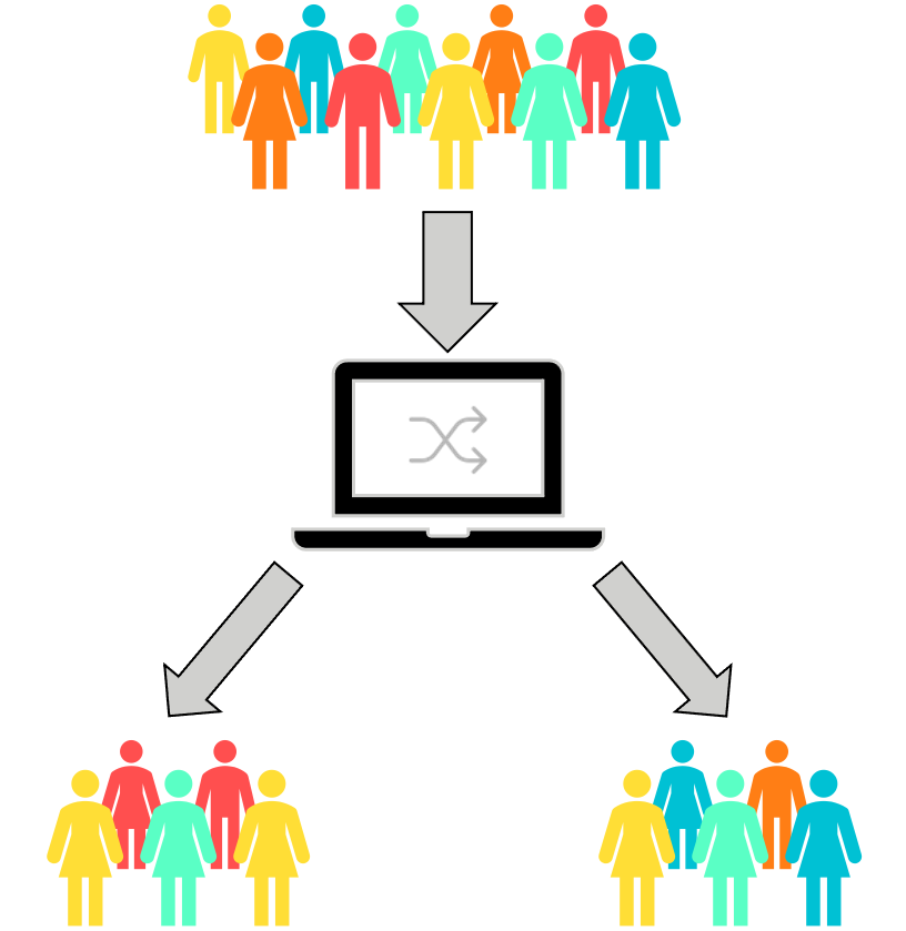
Remember, randomization of treatment should achieve that we are able to interpret the average treatment effect causally and for that, both groups need to be as similar as possible. The image illustrates the randomization process. Try to think what could happen if you have just very few units in both groups. How likely is is that they are very similar regarding their characteristics? You can probably already sense that this might not be sufficient to make groups comparable.

Illustration of randomization process

But let’s try it out and see how average group characteristics develop when we change the sample size.

viewof N = Inputs.range(
  [10, 10000], 
  {value: 10, step: 10, label: "Number of individuals:"}
)

theme = ({
  style: "background-color: #0F2231",
})

mutable yDomain = [10, 100]

Plot.plot({
  ...theme,
  facet: {data: filtered, x: "variable"},
  grid: true,
  color: {legend: true},
  marks: [
    Plot.dot(filtered, {x: "treat", y: "mean", stroke: "#00C1D4", tickSize: 1, fill: "#00C1D4"}),
    Plot.tickY(filtered, {x: "treat", y: "ci_l", stroke: "#00C1D4"}),
    Plot.tickY(filtered, {x: "treat", y: "ci_h", stroke: "#00C1D4"}),
    Plot.ruleX(filtered, {x: "treat", y1: "ci_l", y2: "ci_h", stroke: "#00C1D4"})
  ],
  y: {domain: yDomain}
})

filtered = transpose(data).filter(function(df) {
  return N === df.N;
})

As you can see in the plots, group average characteristics converge with increasing sample size. The more units are assigned to either group, the less differences are between the groups and thus, the independence assumption, stating that groups only differ by their treatment status, is fulfilled. But although you need a minimum amount of units, there is not much improvement after increasing the sample size way beyond that (also, the difference is already really small).

Average Treatment Effect

Just because we can, we use the whole sample. That means there should be about ~500 units per group. There are many suggested rules and guidelines to choose the right sample size, but for now, we will disregard it as our data is simulated and therefore, we do not have any data problems.

So far, we have just looked at the covariate balance but have not included the outcome variable. Let’s do that now. In the background I simulated the outcome after treatment and added the column outcome to our table.

# Show data with outcome variable
df_out

As already mentioned, having balanced baseline characteristics between treatment and control group allows us to estimate the average treatment effect.

But how do we calculate the average treatment effect? We can just take a simple difference in means to estimate it. By the way, groups can be of different group size. It is only important, that they are comparable in their characteristics.

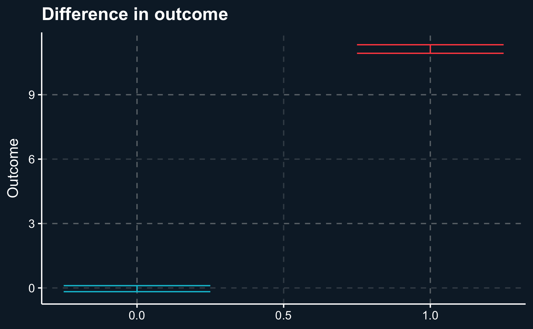
Let’s compute the average outcome per group. We see that there seems to be a difference, the average outcome in the treatment group is higher.

# Group by treatment group and compute average outcome
df_out %>% 
  group_by(treat) %>% 
  summarise(mean_outcome = mean(outcome))

Generally, it is recommendable to use a linear regression to get an estimate of the treatment effect. You don’t have to manually compute the difference and additionally, the output of lm() and summary() yields information to be used for statistical inference. Then, we see that this effect is in fact highly statistically significant. The effect is equal to the difference of the two values just seen above. Check it out (small differences possible due to rounding)!

# Compute ATE with linear regression
lm_ate <- lm(outcome ~ treat, data = df_out)
summary(lm_ate)

Call:
lm(formula = outcome ~ treat, data = df_out)

Residuals:
    Min      1Q  Median      3Q     Max 
-24.207  -4.261  -0.038   4.197  24.837 

Coefficients:
            Estimate Std. Error t value Pr(>|t|)    
(Intercept)  -0.0337     0.0885   -0.38      0.7    
treat        11.1626     0.1246   89.57   <2e-16 ***
---
Signif. codes:  0 '***' 0.001 '**' 0.01 '*' 0.05 '.' 0.1 ' ' 1

Residual standard error: 6.2 on 9998 degrees of freedom
Multiple R-squared:  0.445, Adjusted R-squared:  0.445 
F-statistic: 8.02e+03 on 1 and 9998 DF,  p-value: <2e-16

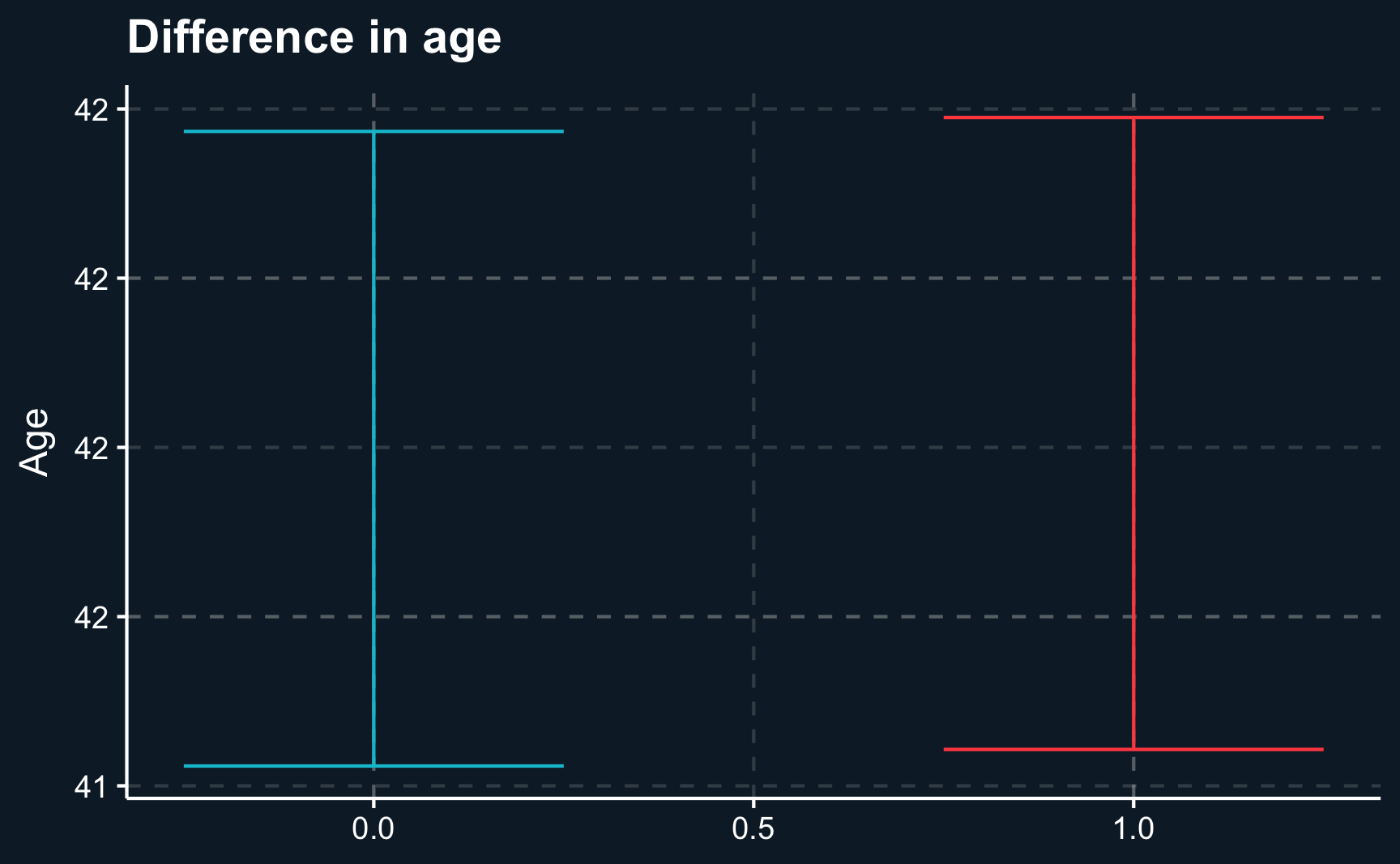
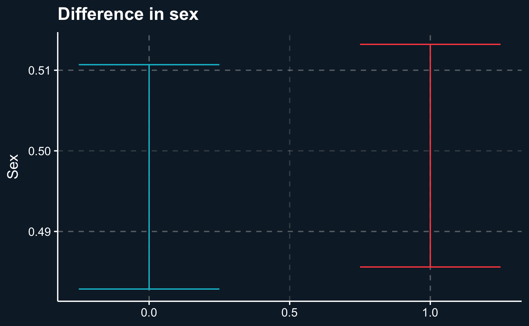
One way to present your results to your audience could be a boxplot that on the one hand shows the difference of regressors by group and on the other hand the difference of outcomes. Here we will show the 95% confidence intervals for our estimates and it can be seen that there is a substantial difference between both groups. However, for our independent variables, age and sex , both groups are very similar.

# Plot independent and and dependent difference
# age (independent)
compare_age <- 
  ggplot(df_out, 
         aes(x = treat, 
             y = age, 
             color = as.factor(treat))) +
  stat_summary(geom = "errorbar", 
               width = .5,
               fun.data = "mean_se", 
               fun.args = list(mult=1.96),
               show.legend = F) +
  labs(x = NULL, y = "Age", title = "Difference in age")

# sex (independent)
compare_sex <- 
  ggplot(df_out, 
         aes(x = treat, 
             y = sex, 
             color = as.factor(treat))) +
  stat_summary(geom = "errorbar", 
               width = .5,
               fun.data = "mean_se", 
               fun.args = list(mult=1.96),
               show.legend = F) +
  labs(x = NULL, y = "Sex", title = "Difference in sex")

# outcome (dependent)
compare_outcome <- 
  ggplot(df_out, 
         aes(x = treat, 
             y = outcome, 
             color = as.factor(treat))) +
  stat_summary(geom = "errorbar", 
               width = .5,
               fun.data = "mean_se", 
               fun.args = list(mult=1.96),
               show.legend = F) +
  labs(x = NULL, y = "Outcome", title = "Difference in outcome")

# Plot age, sex and outcome differences for both groups
compare_age
compare_sex
compare_outcome

Treatment and control group overlap regarding average age.

Treatment and control have similar proportion in terms of gender.

Differences in outcome can therefore be ascribed to treatment variable.

But why did we not include \(age\) and \(sex\) into our regression? Because they are similarly distributed across both groups it should not change the treatment effect. But still, they might have an impact on the outcome, as well. Although being similarly distributed in both groups, they can still vary within each group. So let’s see what happens if we include them.

Both regressors turn out to be significant. However, as expected, the treatment effect is almost unchanged. If there had not been a covariate balance between the two groups, our treatment effect would have been biased.

# Include other regressors
lm_all <- lm(outcome ~ treat + age + sex, data = df_out)
summary(lm_all)

Call:
lm(formula = outcome ~ treat + age + sex, data = df_out)

Residuals:
    Min      1Q  Median      3Q     Max 
-20.987  -3.908  -0.086   3.900  21.746 

Coefficients:
            Estimate Std. Error t value Pr(>|t|)    
(Intercept) -4.70708    0.19990   -23.6   <2e-16 ***
treat       11.14857    0.11324    98.5   <2e-16 ***
age          0.05264    0.00419    12.6   <2e-16 ***
sex          4.98913    0.11324    44.1   <2e-16 ***
---
Signif. codes:  0 '***' 0.001 '**' 0.01 '*' 0.05 '.' 0.1 ' ' 1

Residual standard error: 5.7 on 9996 degrees of freedom
Multiple R-squared:  0.542, Adjusted R-squared:  0.542 
F-statistic: 3.94e+03 on 3 and 9996 DF,  p-value: <2e-16

Subgroup analysis

The significance of \(age\) and \(sex\) could also indicate that there are different treatment effects across different levels of both covariates. Then, a so called interaction/moderation effect would be covered behind the statistical coefficients.

A moderation effect expresses different strengths of the treatment for different subgroups. For example older people might benefit relatively more from the treatment than younger people. And women might benefit more from treatment compared to men.

In R, we include interaction effects by using either using a product x1*x2 or a colon x1:x2. In fact, when we do that, the interactions are significant and the treatment effect changes substantially.

Note, that now the treatment effect differs for everyone dependent on their age and sex. Now it requires a bit of addition to obtain the treatment effect. Moreover, it is not the \(ATE\) anymore, but instead the conditional average treatment effect \(CATE\) as it depends on other covariates.

# Include interaction
lm_mod <- lm(outcome ~ treat * age + treat * sex, data = df_out)
summary(lm_mod)

Call:
lm(formula = outcome ~ treat * age + treat * sex, data = df_out)

Residuals:
   Min     1Q Median     3Q    Max 
-19.19  -3.45   0.02   3.39  18.78 

Coefficients:
            Estimate Std. Error t value Pr(>|t|)    
(Intercept) -0.21009    0.24269   -0.87     0.39    
treat        2.42849    0.34049    7.13  1.1e-12 ***
age          0.00561    0.00530    1.06     0.29    
sex         -0.11579    0.14276   -0.81     0.42    
treat:age    0.08841    0.00745   11.86  < 2e-16 ***
treat:sex   10.10470    0.20116   50.23  < 2e-16 ***
---
Signif. codes:  0 '***' 0.001 '**' 0.01 '*' 0.05 '.' 0.1 ' ' 1

Residual standard error: 5 on 9994 degrees of freedom
Multiple R-squared:  0.639, Adjusted R-squared:  0.639 
F-statistic: 3.54e+03 on 5 and 9994 DF,  p-value: <2e-16

Note also that \(R^2\) has increased with each addition to the regression. But why do you think the main treatment effect is not significant anymore?

As the data is simulated, we can check what the true data-generating process is and based on that evaluate what regression equation provides the best solution. Check for yourself what model should be used.

\[ outcome = 2*treat + 0.1*treat*age + 10*treat*sex + \epsilon \]

Again, it shows how crucial theoretical knowledge of the phenomenon you are studying is. Imagine a situation with a high number of regressors. Testing out all potential variables as moderators requires some effort and might even lead to results just due to chance. You should therefore plan your research design and hypotheses beforehand. As a matter of fact, many scientific publications therefore have to define a pre-analysis plan¹.

Conclusion

In this chapter, you should have learned the benefits of randomization. So why not just always randomize treatment objects and make causal claims afterwards? Although there are some fields like medicine, particularly drug trials, that almost fully rely on randomized controlled trials, other fields cannot rely on RCTs due to a variety of reasons.

For example in social sciences conducting RCTs can be problematic due to high cost or for ethical reasons. One example would be researching the effect of smoking during pregnancy on success of the child later in life or the effect of marriage on wages. It is clearly unethical to dictate some women to smoke during pregnancy as we already know that it will very likely do damage to both mother and children and we are not interested in the direction of the effect but rather in the magnitude. Also, we cannot randomly tell people to get married for obvious reasons.

Another example would be the effect of implementing a minimum wage on some employees. While the result is not obvious in this case, it is still not fair to pay minimum wage only to a selection of the workforce as it substantially affects their life.

Also, many government programs like e.g. unemployment insurance cannot given only to a random sample of people to identify the effect.

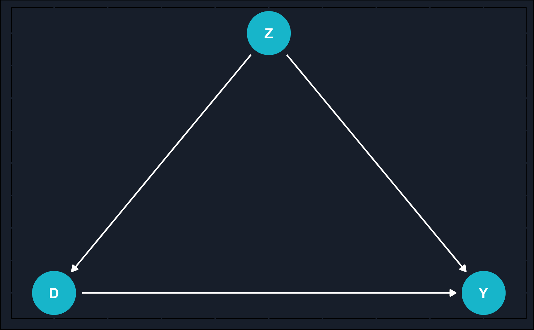
Additionally, in business context, you are also interested in analyzing past data, that has not been collected using randomized settings. In such cases, researchers need to rely on observational studies to estimate effects. Using our graphical language introduced in the previous chapters, let’s illustrate the difference between observational studies and DAGs.

Code

# Load package to draw DAGs
library(ggdag)

# (1) Observational studies
# define DAG
obs_topic_DAG <- dagify(
  D ~ Z,
  Y ~ Z,
  Y ~ D,
  coords = list(x = c(Y = 3, Z = 2, D = 1),
                y = c(Y = 0, Z = 1, D = 0))
)

# draw DAG and assign to object
obs_dag <- ggdag(obs_topic_DAG, node_size = 10) +
  theme_dag_cds() +
  geom_dag_point(color = ggthemr::swatch()[2]) +
  geom_dag_text(color = "white") +
  geom_dag_edges(edge_color = "white")

# (2) Experimental studies
# define DAG
exp_topic_DAG <- dagify(
  Y ~ Z,
  Y ~ D,
  coords = list(x = c(Y = 3, Z = 2, D = 1),
                y = c(Y = 0, Z = 1, D = 0))
)

# draw DAG and assign to object
exp_dag <- ggdag(exp_topic_DAG) +
  theme_dag_cds() +
  geom_dag_point(color = ggthemr::swatch()[2]) +
  geom_dag_text(color = "white") +
  geom_dag_edges(edge_color = "white")

# Plot both DAGs
obs_dag
exp_dag

Observational study

Experimental study

Observational studies are based only on what a researcher observes as opposed to experimental studies where a researcher actively intervenes. In observational studies, one large issue (not the only one) is confounding by other variables. Confounding falsifies our estimate in case we do not control for this variable. Because in many times, we don’t know confounders or they are unobserved, estimates from observational studies always rely on additional assumptions and domain knowledge that randomized experiments do not require.

Opposed to that, in RCTs, there is no arrow from the confounder to the treatment assignment. That is because we randomized treatment and therefore, by construction, treatment selection cannot be confounded. In our example that was indicated by the covariate balance across treatment and control group.

All other tools that we will learn in the following chapters try to deal with the issue of isolating causal effects in observational studies by exploiting the underlying causal mechanisms.

Assignment

Load the dataset abtest_online.rds. It contains data about a randomized experiment run by an online shop. E-commerce websites frequently conduct numerous randomized experiments, commonly referred to as AB testing in a business context. In these experiments, a subset of randomly chosen website visitors is presented with a slightly altered version of the site, while others see the standard version. This approach enables the testing of new features, and the decision to implement a new feature is contingent on the outcomes derived from these tests.

Consider this situation: You operate an online store and are concerned about the expenses associated with your customer service. To cut costs, you contemplate introducing a chatbot as a substitute for human customer service. However, you’re uncertain whether this change might have a detrimental impact on your sales. Consequently, you intend to conduct an AB test. In this test, a portion of users will be directed to a website equipped with a chatbot (treatment group), while the remaining customers will still interact with human customer service (control group) if they have questions. To ensure randomization, you’ll allocate the treatment based on the last digit of each user’s IP address.

There are two outcome variables, purchase and purchase_amount. The first one shows whether a customer bought and the other how much (in €) he bought. First, let’s use purchase_amount.

Other variables included are mobile_device being TRUE when a user visits the site using a mobile device and previous_visits indicating the number of previous visits of a particular user.

After loading the data, perform the following steps:

1. Check whether the covariates are balanced across the groups. Use a plot to show it.
2. Run a regression to find the effect of chatbot on sales.
3. Find subgroup-specific effects by including an interaction. Compute a CATE for one exemplary group. A subgroup could be for example mobile users.
4. It’s not only of interest how much customers buy but also if the buy at all. Then, the dependent variable is binary (either 0 or 1) instead of continuous and the model of choice is the logistic regression. Use the outcome variable purchase and run a logistic regression. The coefficients are not as easily interpretable as before. Look it up and interpret the coefficient for chatbot.

Tip

Use the command glm(formula, family=binomial(link='logit'), data).

How to submit your solutions!

Please see here how you have to successfully submit your solutions. I would recommend you to solve the assignments first in .R scripts and in the end convert them to the required format as explained in the submission instructions.

Footnotes

1. https://blogs.worldbank.org/impactevaluations/a-pre-analysis-plan-checklist